Architectural Resiliency of GNN Algorithms to Graph Structure
A slightly edited version of my project report.
Why is Graph Training Important?
Many complex systems are modeled using graphs such as social networks, transportation networks, recommendation systems, and knowledge graphs, among many others. [1] Along with the rise of artificial intelligence and machine learning, the importance of performing deep learning on these graphs becomes more necessary as time progresses to gain insight into this data. However, graphs have complex and varied structures that need to be interpreted by deep learning algorithms, which gave birth to many convolutional algorithms such as GCN, GIN, and GraphSAGE.[2][3][4] These algorithms detect complex structures inside the graph and perform convolutions to extract features that feed dense layers enabling deep graph learning.
An essential question for architects to explore is how the GNN algorithms and underlying hardware perform relative to changes in the graph structure. This is similar to the need to understand how the number of features affects DNN implementations or how the size of images processed by CNNs affects the utilization of systolic arrays. One step could be to analyze how the number of nodes and edges affects a GNNs performance; however, a more unique aspect of graphs is that they can be structured in various ways, even with the same number of nodes and edges. This project's primary focus is looking into precisely how performance responds to structural changes.
Can we affect the hardware performance of GNN algorithms by modifying the input graph, and why do we care?
The importance of investigating how graph structure affects GNN performance is twofold.
First, the graph structure can change over time. While the growth of a graph in nodes or connections may be predictable, the underlying change in structure may be more unpredictable. For example, you may be able to predict/control the growth rate of products on your platform or users for your app; however, which products are bought with one another or how people use your app is less predictable/controllable. In addition, these graphs can be easily scaled; you only apply the GNN to the X most bought products or the Y most popular users, but filtering connected nodes is more convoluted as the connections themselves provides the information the GNN is trying to capture.
Suppose an architect is developing an ASIC-based system. In that case, it is essential to know how the resource usage and utilization may need to change over time and how the limits of a HW/SW stack respond to changes in the graph either during or after the long development cycle. [5]
Second is adversarial attacks on the graph itself, a topic seen in previous research. [6] While changes in the nodes or edges can be detectable, changing the underlying structure over time could be more brutal to detect and correct. Attacks done over a long time spread over many users can change the underlying structure easily. What was the last time you checked that all of your connections were real?
In addition, GNNs are used to detect fake edges and nodes. If the attack cannot be seen in time, the fraud detection GNN itself becomes unusable as the underlying structure makes it unscaleable.
Overall this project aims to investigate how the structure of a graph affects the performance of the convolutional algorithms processing that graph. This is done by quantizing the graph structure and measuring how much GNN runtime performance changes with small to significant changes. The major causes of this performance change will then be investigated through profiling, and the resulting measurements will help identify how these structural changes affect performance. This project details two specific structure-modifying methods used to identify significant drivers in performance change.
What has been looked into Previously?
Previous studies have investigated how structure fundamentally affects GNN performance and how information inside the graph could affect accuracy [7]. This research focused on how multiple GNN algorithms could handle long and short-range information transfer in graphs. (Whether to classify specific nodes, the GNN needs to know about connections across the graph or just neighboring nodes.) However, this paper only focuses on accuracy and not hardware performance, though it does introduce the concept of specific GNN algorithms being sensitive to the graph structure.
Other studies focus on handling possible adversarial attacks on underlying structures [6]. This paper developed a method to regularize structural information in graphs to get a minimal set of neighboring information needed for accurate results. This paper also simulated changes in graph structure through techniques such as Nettack and random shifting of node features. While focusing on accuracy again, this paper does introduce the concept of gradually changing the graph structure and measuring its effects.
Meta papers also bring up the topic and mention methods that address how graph structure affects the data flow and partitioning of the work, but these papers don't look at the individual GNN algorithms. [5] Overall previous work does investigate how structure affects the accuracy and dataflow of GNNs but not as much into their hardware performance which is what this project tries to address.
How can we describe and quantify graph structure?
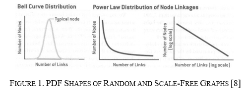
Basic graphs are constructed from two main elements: nodes and edges. Typically graphs contain many nodes, each connected to other nodes through edges. The amount of edges any given node will have is called the "degree" of the node. Plotting the distributions of the node degrees in a Probability Distribution Function gives insight into the underlying structure of the graph. For example, the two graph structures focused on in this report's first part have significantly different PDF shapes.
The two graph structures in this paper are random and scale-free graphs. Random graphs have a degree distribution that looks normally distributed, making the PDF look like a bell curve, as shown on the left in Figure 1. This is because, in random graphs, the number of connections for each node stays relatively in the same range—for example, highways in the United States. Typically highways connect and produce nodes that are only about three to six connections. No set of highways connects to create an intersection with 100 off-ramps. The second structure is scale-free, meaning the distribution of node degrees follows the power law closely, making the node degree more exponential, as shown in the middle of Figure 1. This means that most nodes have a small number of connections; however, there exist hubs that are nodes with a significantly higher degree count. An example of this is air traffic in the United States. Many small airports only have one to ten flights; however, a couple of hubs like Atlanta and Dallas have thousands of flights daily.
To quantify structure for at least the first part of this project, I focused on moving a graph from its original state to a more random state. This is explained more below, but essentially, the graph can be modified from 0 to 100% random from its starting graph, giving us a sliding scale to change the underlying structure.
What GNN algorithms are being used, and how would node degree affect them?
The concept of a Graph Convolutional Network is similar to Convolutional Neural Networks. A feature detection algorithm is run on a small part of the data, and then the algorithm is moved to the next data clump. In the CNN case, the neighborhood is pixels around the target pixel as defined by a filter size, and the movement is the stride to the next pixel to run the filter over. For GNNs, the neighborhood consists of some nodes at least a number of hops away from the target node called a neighborhood, and the stride is the movement to a neighboring node.
As for the GCN algorithms used in this paper, three primary convolutional types are used:
· GCN: an algorithm that extends typical convolutional neural nets to operate on graph-structured data. [2]
· GraphSAGE: an algorithm that learns node embeddings by combining feature information from a local neighborhood of nodes. [3]
· GIN: an algorithm that aggregates data from the neighborhood of a node through graph permutation. [4]
Using these three algorithms is twofold. The first is to see if the performance change seen is algorithm agnostic, in which all algorithms will see similar performance changes. Second, to see if different algorithms may be more or less sensitive to the underlying structural changes.
What benchmarks are being run and using what hardware?
The following experiments were run on a Python 3.9.16 notebook using the Google Collab Suite, specifically the High-RAM Premium GPU instance. This instance consists of an A100-AXM4-40Gb GPU and an Intel Xeon CPU. Pytorch 2.0.0 was used to build and run these models on CUDA version 11.8.
The benchmarks for these experiments were taken from Stanford's Open Graph Benchmark suite, which covers multiple application spaces, three main graph learning tasks, and various graph sizes. [9] For this project, the focus was on node and graph classification tasks. Node classification tasks focus on being able to predict node labels for large graphs; however, graph classification focuses more on classifying smaller graphs as a whole and aims toward graph throughput. This provides coverage for processing a small number of large graphs and a large amount of smaller graphs.
For node classification, the following benchmarks were used:
· ogbn-products: A dataset with 2.4 million nodes and 61 million edges containing information about the relationship between products people buy. The task is to classify products into specific groupings.
· ogbn-arxiv: A dataset with 170 thousand nodes and 1.1 million edges that contains information detailing how academic papers cite one another. The task is to classify papers into subject areas.
For graph classification, the following benchmark was used:
· ogbg-molhiv: A dataset of 41 thousand graphs with an average size of 25 nodes and 27 edges. Each graph represents a molecule's structure, and the task is to identify what molecule a graph represents.
All three GNN models had the same structure of three hidden layers, each with a size of 64 with a dropout rate of 50%. A batch normalization layer was put between each convolutional layer for each model. For the graph classification benchmark, a batch size of 64 was used.
The GCN, GraphSAGE, and GIN implementations were taken from two Git repositories that provide example implementations to run the Open Graph Benchmark.[10][11] These two repositories had slightly different implementation methods, so the comparisons were never made on algorithms implemented in the different methods.
To measure the runtime, FLOPSs performed, and memory allocated, the Pytorch profiler "torchvision" was used. The profiler gave a breakdown for each kernel run on the GPU and all processes run on the CPU, giving a high-level picture of where the time is spent for each run. From trace inspection, it was determined that measuring the time in the "aten::to" CPU process was an excellent analog to memory transfer time. Then the "spmm" kernel time on the GPU was used as an analog to measure GPU computation time. The process memory allocation amount did not have a high enough resolution to represent memory transfer time, as it did not change across runs. In the same vein, the FLOP count was only on the CPU side, which was consistent across runs also; thus, these two measures were avoided. These measurements were used explicitly for the node classification tasks. Graph classification tasks spent time in different processes and kernels, which did not allow for using the above, and the focus was more on CPU computation. Here the ratio of CPU and CUDA runtime was measured along with time spent inside "aten:cat", "aten:narrow", and "aten:embedding" processes which took up the majority of the CPU compute time.
Figure 3 shows the end-to-end setup using the OGB packages. The graph modification detailed in the following two sections is done between retrieving and loading the dataset into the model. Measurements are done on the execution of the model between loading and evaluation.

How is the graph structure being modified, where does that fit in, and what is data being collected?
Once the above is set up and running, baseline results for each GNN algorithm for each benchmark can be measured with no graph modifications. The next step is to modify the graph structure gradually and see how the performance changes relative to the baseline. Two main graph modification methods were used, with the second inspired by results from the first.
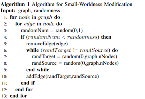
The first algorithm uses a modified version of the "Small-World" algorithm proposed in a fundamental network theory paper. [12] In the paper, this method was used to display how small-worldness affects average clustering and average node distance of a graph, which is outside the scope of this paper; however, this method is suitable for giving a gradual way to change the underlying structure of the graph without adding or removing nodes and edges. The algorithm is as follows:
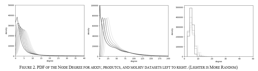
In addition, this allows for modification of the graph without global knowledge, which is advantageous for attacks on a graph. Figure 2 (I know WhY dOEs 2 cOme AftER 3. In the IEEE formatted paper it makes more sense) below shows how the PDF gradually becomes more "random" and less "scale-free" for each dataset by getting closer and closer to a bell curve distribution. The results from running these graphs over these benchmarks show how graph structure affects each GNN algorithm.
From the results of the above experiment, it was theorized that each of the GNN algorithms and use cases might have a node degree to which they are sensitive. More nodes below or above sensitive node degrees may cause significant performance gain or degradation. This hypothesis was tested by sweeping an impulse over the PDF function, as seen in Figure 4 below.
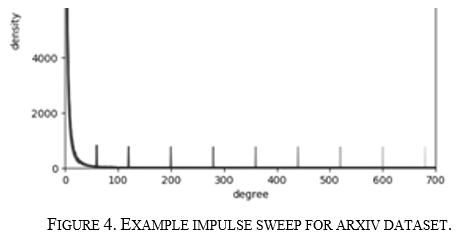
This was done for both node classification tasks; however not done for graph classification as the algorithm used before did not map to how the data is structured for these benchmarks well, and there needed more time to get it running. The following algorithm was run on each graph with a fixed impulse height and a range of impulse degrees:
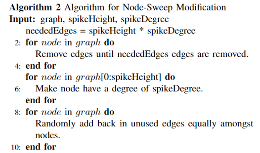
Each graph is run with an impulse at gradually increasing degrees, and the same measurements were performed as done for the small-world modification. An improvement for this could be to have the spike height not be arbitrary, as the spike height affects how much the underlying node distribution needs to change to create the spike; however, if the spike is too small, the effect seen is also too small.
How do GCN and GraphSAGE respond to changes in arvix graph structure?
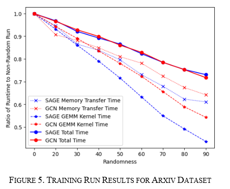
For the training and inference runs, the graph was run for 20% to 90% randomness in steps of 10%. The results show a linear decrease in runtime in all measurements for both the GCN (Red) and the GraphSAGE (Blue) algorithms, as seen in Figure 5 for training and Figure 6 for inference. For GraphSAGE, the GPU Compute time and memory transfer time decreased faster than GCN; however, both total runtimes fell at the same rate. These results point to structural changes to graphs being more model agnostic, but it does display how underlying structure can significantly change performance as it improved up to 20% in both the training and inference cases.

How do GCN and GraphSAGE respond to changes in products graph structure?
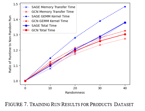
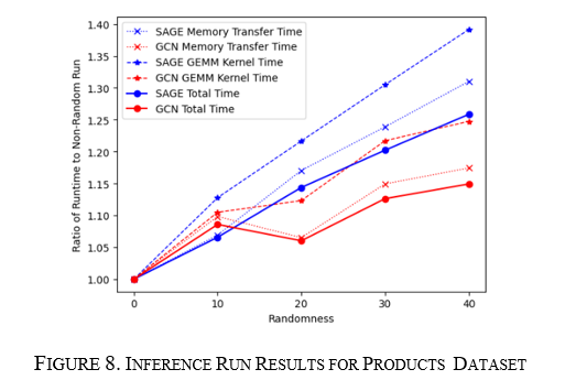
For the training and inference runs, the graph was run for 10% to 40% randomness in steps of 10%. In this case, both GCN and GraphSAGE runtimes increase; however, for training and inference, GCN's increase starts to taper at about 40% versus GraphSAGE's constant linear increase. This is seen in Figure 7 for training and Figure 8 for inference. Here the same thing is seen where the memory transfer and the GPU compute portions increase at the same rate as the overall runtime showing they both drive the change in total runtime.
How do GCN and GIN respond to changes in proteins graph structure?
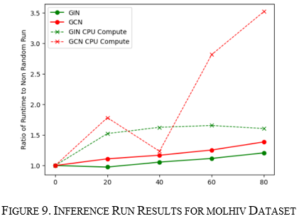
Unlike the previous benchmarks, this benchmark had different results between training and inference. The initial findings show that the performance stays constant for training; however, it gets worse for both algorithms performing inference, as seen in Figure 9. When looking at the traces, the CPU computing processes dominated the inference. This led to me plotting the ratio of CPU compute time versus GPU compute time for both runs. This ratio was seen to be constant for training which had no change in runtimes; however, it gradually decreased for inference, as seen in Figure 10. This points to the fact that inference for these many small graphs starts to be CPU dominant in the linear nature from accumulating results. Further investigation needs to be done to see if batch sizing may contribute to this behavior. The above was seen for both the GIN and GCN convolutional algorithms. However, GCN looks more sensitive.

What has been learned so far, and what still needs to be done?
These initial experiments were interesting as the results, in one way, were similar for all algorithms showing more algorithm-agnostic behavior. However, the total runtime behavior of each benchmark changed entirely to the point that all three had different characteristics. The arxiv showed a performance increase with the increased randomness, products showed a performance decrease in randomness, and molhiv stayed about the same for training and got worse for inference with increased randomness. When zooming in on the PDF modifications, as seen in Figure 11 below, it can be seen that the randomness caused similar changes to the underlying structure. From this, it can be inferred that each algorithm may have different node degree points where they are sensitive.

For arxiv, where the performance improved, the sensitive node degree might be at a point where the number of nodes at that degree is decreasing, as seen on the left; for products that node degree could be at a point where the number of nodes is increasing as illustrated on the right; and for molhiv, the structure changed a relatively small amount seen in Figure 2 so all of the graphs may be blow a theoretical sensitive node degree.
This leads to the next half of this project. To find these sensitive node degrees, I swept a spike across the node degree pdf function. Ideally, I wanted a constant change with certain points having a slope change; however, we will see that is not quite what happened.
How does the node sweep affect arxiv?
For the node sweep, the experiment was focused on the training runs as the inference and training runs followed one another for the Small-World experiment and to save some compute resources. The sweep was done from a node degree of 50 to 700 in increments of 10, and the height of the moving impulse was 750. The runtime was similar to the Small-World runs in that both GraphSAGE and GCN moved together at the same points; however, GCN varied more, as seen in Figure 12 below, which aligns with what was seen previously with GraphSAGE being more agnostic to change.
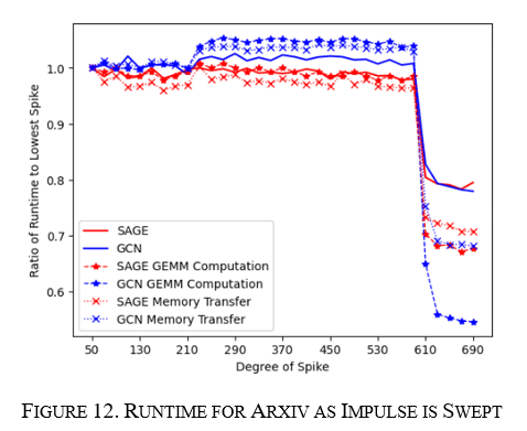
The shape of the runtimes was not uniform as was expected; instead, there were disjoint sections in the graphs at specific degrees. Up until 250 degrees, the performance was relatively flat, then jumped and stayed relatively flat until a degree of 550, then significantly dropped by about 20%. This behavior is illustrated in Figure 12.
This overall points to two things:
· These GNN algorithms are sensitive to structure, and there exists a mechanism that can significantly affect runtime. We need to find out what occurs at these inflection points causing large jumps in change.
· The non-uniform slope points to this algorithm not doing an excellent job of keeping the underlying structure the same when making the impulse. It's possible the change from the algorithm is very nonlinear, as the number of nodes needed to create the spike changes greatly in the higher node degrees. One experiment could be to have the number of edges modified the same but have the spike height change.
How does the node sweep affect products?
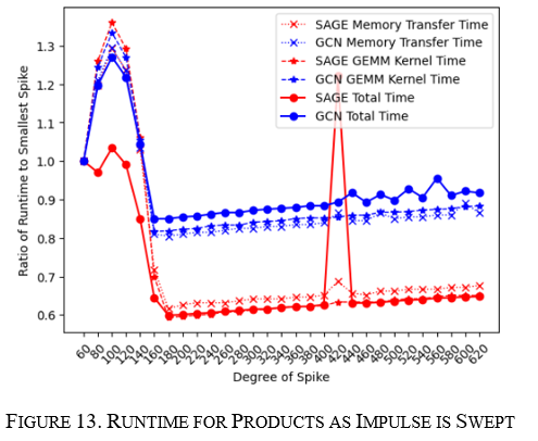
The products impulse was swept from a node degree of 60 to 620 in increments of 10. This showed a similar story as arxiv with an initial jump and then a significant dropoff later on; however, this node sweep was longer and showed progressively increasing runtimes as the degree of the spike approached 620, as seen in Figure 13 below. In addition, the variability of the GCN algorithm was more significant than GraphSAGE showing a more considerable initial jump and a more significant drop in runtime later on.
What about molhiv?
The algorithm I made didn’t work as well on molhiv making the spike not as significant. I would propose exploring another method to investigate smaller graphs.
What have we truly figured out?
These experiments show that graph structure significantly impacts the convolutional algorithms' performance even though no nodes or edges were added or removed. GraphSAGE, GCN, and GIN were affected the same in these experiments, except that they have different sensitivities to the modification in the graph structure, pointing to these changes being more algorithm agnostic but very sensitive to the particular algorithm. Overall, if the underlying graph is dynamic, it is wise to research an appropriate convolutional algorithm insensitive to graph structure changes and have hardware that can handle it. More research needs to be done to see what precisely the hardware has to do to handle it.
Not detailed above, but I also graphed how neighborhood size changes with each of these graph modifications. I saw that they all had the same pattern of the neighborhood size shrinking with a distance of 2 for all the graph modifying algorithms; however, when I presented this to some of my colleagues, a good point was brought up that it may be more related to the placement in memory of the nodes in the neighborhood versus the size of the neighborhood itself—another good place to have some further research.
Whereas the memory transfer size and GEMM computation time correlate and move together, pointing to a difference in size for the GEMM computation that is needed based on the graph structure—however, a direct relationship to how the size of the GEMM computation changes with structure was not found and could be further researched.
What does this lead into?
The future work can be done in many directions:
In both experiments, it was seen that the network structure could greatly reduce the runtime of the convolution. An interesting topic would be to isolate this mechanism and see how it affects the training rate and accuracy. If minimal, this may be an optimization that could lead to faster training and inference for the cost of some accuracy if the accuracy goes down.
A broader survey of GNN algorithms to their sensitivity to changes in graph structure could give a better idea of how to categorize algorithms based on sensitivity. For example, GCN algorithms can be labeled as Spectral or Spatial. It would be interesting to see if these meta-groupings have any effect.
Further investigation into the mechanisms which cause this change in runtime could give insight into how to address this sensitivity and possible attack vectors if there was data manipulation.
What are my sources?
[1] J. Zhou, G. Cui, Z. Zhang, C. Yang, Z. Liu and M. Sun, "Graph Neural Networks: A Review of Methods and Applications," in CoRR, vol. abs/1812.08434, 2018. [Online].
[2] Kipf, T. N., & Welling, M. (2017). Semi-supervised classification with graph convolutional networks. ICLR 2017
[3] W. L. Hamilton, R. Ying, and J. Leskovec, "Inductive Representation Learning on Large Graphs," CoRR, vol. abs/1706.02216, 2017. [Online].
[4] Xu, K., Hu, W., Leskovec, J., & Jegelka, S. (2019). How powerful are graph neural networks?. ICLR 2019
[5] S. Abadal, A. Jain, R. Guirado, J. López-Alonso and E. Alarcón, "Computing Graph Neural Networks: A Survey from Algorithms to Accelerators," CoRR, vol. abs/2010.00130, 2020. [Online].
[6] T. Wu, H. Ren, P. Li and J. Leskovec, "Graph Information Bottleneck," in Advances in Neural Information Processing Systems, vol. 33, H. Larochelle, M. Ranzato, R. Hadsell, M. F. Balcan and H. Lin, Eds. Curran Associates, Inc., 2020, pp. 20437-20448. [Online].
[7] U. Alon and E. Yahav, "On the bottleneck of graph neural networks and its practical implications," arXiv preprint arXiv:2006.05205, Jun. 2020.
[8] A.-L. Barabási and E. Bonabeau, "Scale-free networks," Scientific American, vol. 288, no. 5, pp. 60-69, 2003. doi: 10.1038/scientificamerican0503-60.
[9] W. Hu, M. Fey, M. Zitnik, Y. Dong, H. Ren, B. Liu, M. Catasta, and J. Leskovec, "Open Graph Benchmark: Datasets for Machine Learning on Graphs," arXiv preprint arXiv:2005.00687, 2020.
[10] SNAP Group, Stanford University, "Node Property Prediction with OGB," GitHub. [Online]. Available: https://github.com/snap-stanford/ogb/tree/master/examples/nodeproppred.
[11] SNAP Group, Stanford University, "Graph Property Prediction with OGB," GitHub. [Online]. Available: https://github.com/snap-stanford/ogb/tree/master/examples/graphproppred/mol.
[12] D. Watts and S. Strogatz, "Collective dynamics of 'small-world' networks," Nature, vol. 393, pp. 440-442, 1998. DOI: 10.1038/30918.
Thanks for reading! and as always, if you see anything wrong or want to discuss, feel free to reach out.