Leveraging Binary Neural Networks for Efficient Malware Detection

Abstract 

The increasing complexity of networks has given rise to a slew of potential malware attack vectors, whether through infected files, phishing links, or internal agents. Most of this malware includes communication through the network to some control center to get commands for operation and to send sensitive data. As traffic and the variety of malware increases, monitoring this traffic efficiently becomes a dire issue. Machine learning provides some great methods to monitor network communication; however, for a model to be precise in detecting malware and not allow false negatives, it must be complex making it computationally intensive. This report explores the feasibility of using a reduced, more efficient model to filter out the most benign data, lessening the amount of data the complex model must run. This paper proposes a feature reduction methodology and binary neural network model, which, using a FINN BNN accelerator on a 200MHz FPGA, can reduce processing time by approximately 100x for similarly performing models. This model could filter out 68% of the benign test data with only a 0.8% false negative rate. This means that 68% of web traffic can be reliably filtered out with a model that runs with orders of magnitude higher efficiency compared to the larger models.

Introduction 

Modern-day research has looked significantly into how machine-learning models can detect malware attacks based on network traffic. These models primarily operate at a higher level in software that captures incoming traffic and uses a mechanism to put packets into flows which are then processed, as processing on each packet will be very computationally intensive. This paper will use CICFlowMeter, which captures web traffic and puts it into flows of about 85 features. [2]

The critical shortcoming of this methodology is twofold. Many of these high-level models look at features that do not have bounded ranges. This makes it complex for a performance monitor to imitate, as for this project, the flow characteristics must be found and processed in hardware. Second, running large complex models at every endpoint accumulating these flows becomes computationally expensive and inefficient. The inefficiency shows up because these models run on mostly benign data, meaning that in the average case these models use power processing for mostly harmless traffic. In the example dataset, over 70% of traffic is benign. [3] 

This project explores a method in which a significantly smaller and more efficient model can be made using quantization, namely a binary neural network. A binary neural network is a typical multi-layer perceptron model with the exception all weights and values are a binary value, 0 or 1. This means the internal multiply and accumulates can easily be mapped to an XOR and bitcount, which map nicely to an FPGA and hardware in general. 

However, feature reduction methods must be explored to reduce the feature complexity even with this smaller model. For example, suppose the input of this model was 32-bit floating point numbers like the features of the original data set. In that case, the BNN must either quantize the input or have larger Multiply Accumulates (MACs) in its first layer. This means that the feature reduction method must reduce the feature space and quantize the inputs to be a single bit. With reduced features, this smaller model can fit on an independent FPGA, which can be put further up the network to filter out benign data to many clients and mark flows that would need to be analyzed by the larger models. Figure 1 below shows how this FPGA would sit and spy traffic to and from outside networks to alert the victim network of possible malware. Later in the conclusion section, a possible side-channel attack is explored, which would need to be considered.

Figure 1. System Diagram

Motivation

Many recent works have used deep learning for malware detection such as Weitkamp et. al. which looked into ANN, CNN, CNN2D, LSTM, and CNN_LSTM models which were able to get up to 100% accuracy. [5] However, an important point is that the paper used significant hardware (i9 and a GTX2080) but also had relatively long inference times from 0.056 to 0.226ms per row, which is about 4k to 17k flows per second. In addition to Zhou et. al. looked more specifically at 1D CNN networks, which used an i5 with 16GB of RAM to run models that got up above 99.9% accuracy. [7] While these models were able to get good performance, the complexity of the model begs the question of whether they are efficient to run on all web traffic. This work does not aim to replace these models but rather create a small model that can significantly reduce the amount of data these larger models need to run. In addition, the model proposed in this project does not focus on accuracy; rather, what is the largest number of flows that can be filtered for the lowest false negative rate. False positives are not as much of a concern

Sidenote: After I did this project, we had a class (separate class) lecture about weightless models, specifically ULEEN. These are weightless neural nets, and they have had a lot of success in this exact space, having an even more reduced model than BNNs. So I suggest looking into ULEEN and LogicWiSARD. However, it might be more difficult to find packages to get started in terms of training and implementation than BNNs at the moment, as it's more on the edge of research. 

Solution Architecture 

Objectives

The first focus of this project is feature engineering. The objective is to get the features in a format easily generated by hardware and read by the BNN model. In general, it is difficult for hardware to keep detailed running statistics, primarily regarding multiple averages, numbers with wide ranges, etc. However, histograms and binning are commonly used methods for performance monitoring through hardware counters. Thus, this project proposes a way to transform features into bins. With binning, the inclusion of a specific flow is just a 1 or 0, which feeds nicely into a BNN and requires no re-quantization, so the BNN can be contracted purely of XORs and bitcounts, keeping it minimal in size. 

Data Collection

The first step was to find well-labeled benign and malicious data, which was found on the University of New Brunswick's site, "Intrusion Detection Evaluation Dataset." [3] The collection method involves a setup attack network of about four computers with various operating systems and a victim network of multiple routers, switches, and endpoints containing multiple operating systems. Over eight days, numerous attacks were performed, including Web Based, Brute Force, DoS, DDoS, Infiltration, Heart Bleed, and Bot Scan Attacks. The web traffic over a link connecting these two networks was monitored and processed into flows labeled benign or malware if they were related to the attack. Each flow contained about 85 features, which summarized the traffic seen in the flow. Table 1 below describes the data sets included in the complete data set. The "Clean" and "Web Attacks" data set was excluded from training to test the model's performance on unseen data.

Table 1. CIC-IDS2017 Datasets

 Feature Engineering

For the feature analysis, the data is separated by day, where a specific attack is performed each day. Two analysis paths were done to find an optimal way to train data on multiple attack vectors and see if we can take advantage of this split data. The first analysis method is to find the highest correlated features for each attack vector and then combine these sets of features into a master set of features. The second method merges all attack data and finds the features most correlated with the combined attacks. The first method may be better for detecting known attacks. However, the second method might be better for unknown attacks, not overfitting for the specific attacks seen. 

The first step was performed the same for both methods. For each feature, the data's first, second, third, and fourth quartiles were found and stored for later processing. These quartiles will be used to transform each feature into a reduced categorical data set to reduce dimensionality later. 

The next step is to address the skew in the data because, for each set, it was significantly biased against more malicious flows. The skew in the data was the following: 43%,1.23%,44%,1%,0.01%,3.1%, and 36.4% malicious. This skew can significantly affect training, especially if we target a low false negative rate and have a limited amount of positive flows. To address this, SMOTE was run on each data set, creating artificial data to make all used data sets 50/50 benign and malicious flows. 

Next using the quartiles found before the SMOTE step, each data point in each column was replaced by "FIRST", "SECOND", "THIRD", or "FOURTH" depending on what quartile that value was in. If the THIRD quartile finished at the value 0, then the end value was changed to the mean of the feature. This reduces data loss if all data is in the FOURTH quartile. So, instead of all data being thrown in "FOURTH" automatically, it was split on the mean between "THIRD" and "FOURTH."

Once all data is categorized, each column is split into dummy columns. This means that each category-quartile combination has a column, and the row values are either 1 or 0. For example, FlowRate is split up into FlowRate_FIRST, FlowRate_SECOND, FlowRate_THIRD, and FlowRate_FOURTH. Then, one of these columns will have a 1 to indicate which quartile that row was in for that feature. So, from end to end, a feature that started as a floating point number of some arbitrary range is now a set of four features that are mutually exclusive binary numbers. 

Multiple data sets were created from this analysis. First off, the "Clean" data set and the "Web Attack" test data set were saved to their own files. The test data set will be used to see how the models perform on attacks not seen inside the training data. The clean data set will be used to test the false positive rate during normal execution. Next, each day is saved into two sets, pre and post-SMOTE modification. The post-SMOTE will be used for training. However, pre-SMOTE will be used for final analysis as that is the distribution seen in the real world. 

Model Creation

Tensorflow and the Python package larq were used to create the BNNs. [1] Both feature collection methods use the same architecture, which is the following: a Binary Dense Layer with 1024 neurons, Batch Normalization, Binary Dense Layer with 512 neurons, Batch Normalization, Binary Dense Layer with 64 neurons, Batch Normalization, and a Binary Dense Layer with 1 neuron. Each layer used "ste_sign" quantization for the input and output with "weight_clip" kernel constraint. An SGD optimizer was used to build the model. (See https://docs.larq.dev/larq/ for more info about the quantization and the constraints). A trained model will be created for each set of features for each method, resulting in ten overall trained models. More information about how the sets of features are made is in the next section.

To evaluate performance on each model, the preSMOTE data, the clean data, and the test datasets will be used to calculate accuracy, precision, recall, and false-negative rate over a range of thresholds. In addition, an equivalent model was found in the FINN paper to evaluate implementation metrics. It contains metrics such as latency, throughput, and power it takes to run that BNN on the accelerator. These metrics can then be compared to models typically run on CPUs or GPUs.

Table 2. Binary Neural Net Layers

Experimental Results 

Top Features Data by Day 

For method 1 we find the highest correlated features per day. The features are listed in order of correlation to the target variable, which is the malicious/benign label.

Day 1 : Init Win bytes forward FIRST, Fwd Packet Length Max SECOND, act data pkt fwd FIRST, Fwd Packet Length Mean SECOND, Avg Fwd Segment Size SECOND

Day 2 : Init Win bytes backward SECOND, PSH Flag Count FIRST, PSH Flag Count SECOND, Max Packet Length FIRST, Total Fwd Packets FIRST

Day 3 : Init Win bytes forward THIRD, Init Win bytes backward FIRST, Init Win bytes forward FIRST, Bwd Packet Length Min SECOND, Bwd IAT Std THIRD

Day 4 : Active Min FOURTH, Active Mean FOURTH, Active Max FOURTH, Fwd Packet Length Std FOURTH, Avg Bwd Segment Size SECOND

Day 5 : Init Win bytes backward THIRD, min seg size forward THIRD, min seg size forward FIRST, Fwd Packet Length Std THIRD, Bwd Packet Length Min FIRST

Day 6 : Min Packet Length FIRST, Bwd Packet Length Std FOURTH, Packet Length Variance FOURTH, Packet Length Std FOURTH, Bwd Packet Length Max FOURTH

From this we will create 5 sets of features. The first set will take the top 1 from each say, the second set the top 2, the thrid set the top 3, etc..

For method 2 we find the highest correlated features on the overall dataset.

Top Combined Data Features : Min Packet Length FIRST, Bwd Packet Length Std FOURTH, Packet Length Variance FOURTH, Packet Length Std FOURTH, Bwd Packet Length Max FOURTH, Max Packet Length FOURTH, Bwd Packet Length Mean FOURTH, Avg Bwd Segment Size FOURTH, Average Packet Size FOURTH, Packet Length Mean FOURTH, Bwd Packet Length Min FIRST, Fwd Packet Length Min FIRST, Flow IAT Mean FOURTH, Flow Packets FIRST Fwd Packets FIRST, Fwd IAT Mean FOURTH, Idle Mean FOURTH, Idle Max FOURTH, Fwd IAT Max FOURTH, Flow IAT Max FOURTH, Flow IAT Std FOURTH, Idle Min FOURTH, Fwd IAT Std FOURTH, Init Win bytes backward THIRD, Init Win bytes forward FIRST, Flow Bytes/s SECOND, Flow Duration FOURTH, Fwd IAT Total FOURTH, Bwd Packet Length Min FOURTH

From this we will create 5 sets of features. For each set we will take the top x amount of features where x matches the respective method 1 set. For example in the first set method 1 has 6 features, so the first set for method 2 will take the top 6 features.

See https://www.unb.ca/cic/datasets/ids-2017.html for more info about the categories.

Feature Selection Statistics

After the feature sets were found, logistic regression was created using each feature set as the independent variable and the malicious label as the dependent variable. This provided information about the features of the model. The idea is that feature reduction should also make the features more significant and not only reduce the dimensionality of the model for the sake of scaling. Table 3 shows that the feature reduction significantly reduced multicollinearity with more features with smaller VIF scores. In addition higher significance with an increased overall F-Statistic (F-Stat) and larger number of features which are individually deemed significant (P>|t|). At the same, the adjusted R squared shows the cost of using a smaller number of features, which greatly affects method 2.

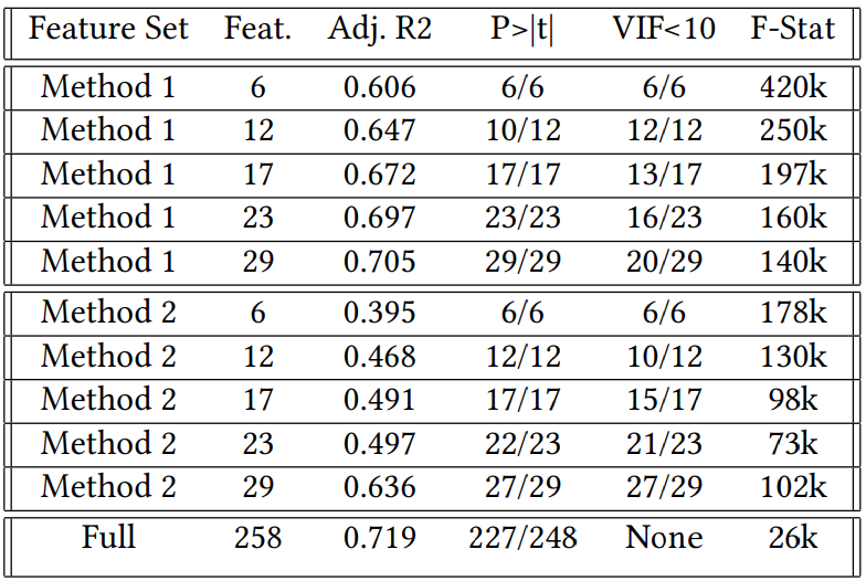
Table 3. Feature Set Characteristics

Method 1. Separated Data by Day

The training was performed over 2.9 million data points with a 33% train test split, with a learning rate of 0.00001 and a batch size of 32, over 32 epochs. The training showed well-behaved results for BNN training as the train and validation acc/auc consistently stayed near one another, showing that the model had relatively good complexity for the problem. In addition, as the number of features increased, the model's performance increased, showing that the feature selection did a relatively good job of adding significant features as the feature set grew.

Table 4. Method 1 Training Results Across Feature Sets

Figure 2. AUC verses Epoch for Method 1

False Negatives on Unknown Attack

Most Method One models could have done better on the unknown attack. Out of a worst-case 1.2% False Negative rate, most models outside the Top 1 model could not reliably detect the attack. However, using low thresholds for Top-1 did detect it with a 0 False Negative rate. Overall, it is also not a positive sign as the metric did not get better as the feature set increased.

Figure 3. False Negative Verses Thresh. for Test Attack

False Negatives on Known Attacks 

These models did better for known attacks. Most models stayed under a 1% false negative rate for over 2.1 Million flows consisting of about 27% malicious traffic. This also showed better behavior, as when the feature set increased, so did the false negative performance.

Figure 4. False Negative Verses Thresh. for Trained Attacks

The threshold of 0.48 was selected as its the largest threshold for the lowest false negative rate. In addition, the Top-5 model was chosen as it had the best performance when addressing known attacks. Table 5 shows the final filter and false negative metrics when running that model on the pre-SMOTE data sets of known attacks.

Table 5. Method 1 Filter Rate and False Negatives

This shows that over half of the traffic could be filtered with a minimal false negative rate of less than 1%. However, this performance was only possible based on data the model had already seen, meaning it would be vulnerable to new attacks.

Method 2. Combined Data 

The training was performed over 2.9 million data points with a 33% train-test split, a learning rate of 0.000001, and a batch size of 32 over 32 epochs. (Same as method 1). The training for this method behaved worse as it was quite noisy for the smaller datasets. One good point is that the training and test performance stayed near one another, pointing to balanced fitting. 

Table 6. Method 2 Training Results Across Feature Sets

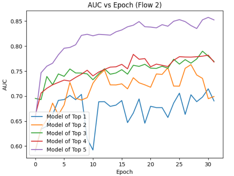
Figure 5. AUC verses Epoch for Method 2

 False Negatives on Unknown Attack

The models for method two proved to work very well for the unknown dataset. For some models and thresholds, it performed near perfectly when filtering out the malicious flows, with a false negative rate of less than 0.1%.

Figure 6. False Negative Verses Thresh. for Test Attack

False Negatives on Known Attacks

Method 2, however, could not perform well for known attacks, with the minimum false negative rate being 7.5% compared to method 1's less than 1 percent. These results point to the possibility of combining these two models to create a mixture of experts. Method 1 to detect known attacks and Method 2 to detect unknown attacks.

Figure 7. False Negative Verses Thresh. for Trained Attacks

Using the same criteria as method one, the Top 2 model with a threshold of 0.88 was used as that had the best performance on known attacks.

Table 7. Method 2 Filter Rate and False Negatives

Method two did not perform as well, filtering just over half of the traffic with a relatively high false negative rate of 7.5%. However, it was able to do this with under half of the features that method one used.

Throughput

About 2.2 Million Flows are processed in 60 to 300 seconds, corresponding to about 36k Flows/Sec and 7k Flows/Sec. This is on the low side performed on a Xeon 2-Core 2.3GHz, and, on the high side, can be run on a V100 GPU High-Ram instance in Google Collab. These are some baseline statistics if one implements these on CPU/GPU hardware. However, the intention is to run on an FPGA. 

Referencing the FINN paper, an equivalent size model would be the SFC-max model. [4] The SFC-Max has 4x 256 neuron layers with a 784-bit input corresponding to 600k OPs, similar to this model. The fundamental similarity is that these two models have the same depth and are close to the same overall OPs. SFC-Max ran at 0.31uS latency with 12361k Frames per second (Flows per second). Running this model in 0.267s for 3.2 million flows beats significantly all models proposed in the CIC-IDS2017 paper and other referenced papers. The FINN paper was made in the same year as the CIC-IDS2017 models, so I believe direct comparisons are appropriate.

Related Work

Table 8 compares the two BNN models created against the baseline models explored in the initial CICIDS2017 paper and three more recent complex models. These three recent models do not have all of these measures in their respective papers; however, they demonstrate the increased performance and longer run times. However, note that the HexCNN performance is not on the CIC-IDS data set but rather a parallel data set from UNB, and it is run on PCAP files, not flows. The ANN and CNN_LSTM times are estimated from their one flow run, so they could get more throughput from batching. 

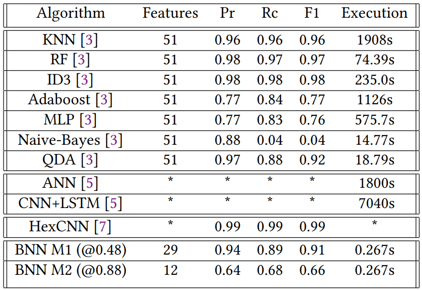
Table 8. Comparison to CIC-IDS2017 and Other Models

A significant work that helps enable the ability to have a reduced model run on features that contain more significant information is FlowMeter [2]. This software summarizes traffic seen in PCAP traces to higher-level flows where each flow has individual features. However, as described before, much of this behavior can be done in hardware in a more quantized fashion. There are also many works related to the use of BNNs on FPGAs. [6] [4] Not only do they provide motivation and insight into the effectiveness of BNNs, but they show that they can significantly reduce model size compared to an almost equivalent larger model in terms of performance. For example, Table 2 and Table 3 of FINN provide some timing numbers for different model sizes, which are achievable with models similar to the one made in this paper

Conclusions

Security Flaws

Toward the end of this project, I did think of one possible side-channel attack. For example, if the victim network is a cloud provider, and the BNN is trained on all traffic of the entire cloud network (or a subsection). Then, a malicious agent running on a VM could gain access to the generated alerts; those alerts, in combination with custom traffic, could leak characteristics of traffic seen by other VMs or nodes in the network. So, if a system like this is used with untrusted VMs, there will probably need to be an effort to hide this alert to some privileged level.

Final Thoughts 

In conclusion, this paper was able to reduce the 85 floating point features seen in CICFlow to 29 (method 1) and 12 (method 2) binary features. These features fed a BNN, which, at best, showed it could filter out 68% of benign traffic with a smaller than 1% false negative rate. By creating this model to be similar to the one described in the FINN paper, this paper could show that the BNN is orders of magnitude faster and more efficient than the larger models recently made and the models originally run in the CIC-IDS paper. However, the main limitation is that this well-performing model needs help performing well for unseen attacks. Future work could investigate if the more general method 2 model could be combined to make a mixture of expert models that can perform well overall. 

References

[1] L. Geiger and P. Team. Larq: An open-source library for training binarized neural networks. Journal of Open Source Software, 5(45):1746, Jan. 2020. 

[2] A. Habibi Lashkari., G. Draper Gil., M. S. I. Mamun., and A. A. Ghorbani. Characterization of tor traffic using time based features. In Proceedings of the 3rd International Conference on Information Systems Security and Privacy - ICISSP, pages 253–262. INSTICC, SciTePress, 2017. 

[3] I. Sharafaldin, A. H. Lashkari, and A. A. Ghorbani. Toward generating a new intrusion detection dataset and intrusion traffic characterization. In 4th International Conference on Information Systems Security and Privacy (ICISSP), Portugal, January 2018.

[4] Y. Umuroglu, N. J. Fraser, G. Gambardella, M. Blott, P. H. W. Leong, M. Jahre, and K. A. Vissers. FINN: A framework for fast, scalable binarized neural network inference. CoRR, abs/1612.07119, 2016. 

[5] E. Weitkamp, Y. Satani, A. Omundsen, J. Wang, and P. Li. Maliot: Scalable and real-time malware traffic detection for IoT networks, 2023. 

[6] Y. Zhang, J. Pan, X. Liu, H. Chen, D. Chen, and Z. Zhang. Fracbnn: Accurate and fpga-efficient binary neural networks with fractional activations. CoRR, abs/2012.12206, 2020. 

[7] Y. Zhou, H. Shi, Y. Zhao, and [et al.]. Identification of encrypted and malicious network traffic based on one-dimensional convolutional neural network. Journal of Cloud Computing, 12(53), 2023.