Lambda Set: A collection of representative graphs for benchmarking.

Abstract— Graphs are essential in many technical fields, such as computer science, and non-technical fields, such as biology and economics. With them being a prevalent workload, there is a need to understand how hardware performs as graphs scale and change structure. However, finding graphs to benchmark on hardware leaves much to be desired. Methods such as selecting a set of real-world graphs, a set of generators, or ones used in previous works open many questions of how representative the set of graphs chosen really is. If one cannot understand how the hardware performs processing various graphs, there can be holes and a lack of understanding, which can be costly when untested workloads are run on an ASIC. This article proposes a suite of graphs that hardware can run to understand how it will perform on the assortment of graphs it might see when running real workloads. This will be done using a complex graph generator that in previous work was seen to generate graphs with structure in many categories involving random, dense, scalefree, star, and sparse. The results of this article show that a selected suite of ten graphs from this generator can represent the performance of many real-world graphs, with the correlation between a selected graph and the real-world graph in all cases is significant and, in almost all cases, significantly correlated with an R2 above 0.85.

I. INTRODUCTION

Many complex systems are modeled using graphs such as social networks, transportation networks, recommendation systems, and knowledge graphs, among many others. [1] Alongside these application spaces are numerous algorithms used to extract information and analyze these graphs, like Breadth First Search, Shortest Path Finding, and Clustering Analysis. [7] The time it takes to perform these algorithms quickly scales up as graphs get large or the algorithms become complex. With the rise of use cases and algorithms, there is a need to understand how well hardware performs on various graphs so that advances in computer architecture and microarchitecture can handle this increase in complexity. However, the variety of use cases presents a problem regarding what workloads the hardware should run to measure the performance of graphs it might see in the real world.

Many routes can be taken to measure hardware performance for these graph applications in research. One route is to select several representative real-world graphs from a database like SNAP [6]; however, that raises the question, How many do you need to choose? Moreover, which ones should be selected to have a representative set? Another route can be to use graphs found in previous work to compare against; however, what happens if the hardware performs better on a set of graphs not included in previous work? Alternatively, what happens when previous work includes graphs deemed unrealistic? In a literature survey, I conducted earlier this year when the same application and hardware space were researched, there was still inconsistency in the graphs used to benchmark the workloads. A few graphs were added and removed with each new architecture evaluation without explaining why they were selected.

Classic graph generators like Erdos-Renyi (Random) [8], Watts–Strogatz (Small World) [9], and Barabasi-Albert (Scale Free) [10] have their limitations. They can only produce graphs of a specific structure, which raises the question of how to generate a complete set using these generators. Previous work, such as RTG, has attempted to address this by creating a unified generator to produce various graphs. However, even these generators require careful parameter selection and can be challenging to match to specific real-world graphs. [5]

The variety of choices needed when choosing what graphs to measure workloads gives a moving target for hardware performance measurement. As brought up by Lord Kelvin, "When you cannot measure it, when you cannot express it in numbers, your knowledge is of a meager and unsatisfactory kind;" [3] This non-standardized way of measuring makes it challenging to gain a genuine satisfactory understanding of how well the hardware architecture and microarchitecture are handling these graph-based applications.

This article proposes a benchmark set of graphs called the Lambda Set, a representative set of graphs that do not have any needed selection of parameters while giving a variety of structures. In addition, it can be back annotated to real-world graphs, meaning this set can be used to derive a method to generate smaller graphs that would imitate the performance of larger graphs. This set of graphs will be constructed using a complex graph generator proposed in "Optimization in complex networks" [4]. This generator has a single parameter lambda that is swept from 0 to 1 and can generate various graphs from scalefree, exponential, random, star, and dense graphs. This article will show that the set of graphs covers structures seen in the real world and that the graphs generated have performance correlated to the real-world graphs, meaning they can be used to model their performance.

The article is organized as follows,

• Section II: Explores previous work in graph generators and establishes the needed characteristics of a generator to benchmark graphs.  

• Section III: Provides background on the network theory used and explains the graph generation algorithm.

• Section IV: Discuss the implementation of the complex graph generator and how the generated graphs will be selected and evaluated.

• Section V: Highlights how well the generated set of graphs covers real-world graphs, which graphs were selected to be in the final set, and how well that final set correlates to the set of real-world graphs.

• Section VI: Discuss the conclusions and future work

II. PREVIOUS WORK

This problem in graph benchmarking has been seen before. It was recently discussed in a paper titled "SoK: The Faults in our Graph Benchmarks," published on arXiv in March of this year. [2] This paper dives into a twelve-year study of benchmarks used in published papers. It found that fewer than 5% of datasets were used in more than ten papers, so selecting the same graphs as previous work has become impossible with time. It also cited how, even when choosing the same benchmark, a dataset titled "Twitter" can have many sources and sizes, causing measurement variability. This paper even found that some datasets used that were deemed illegal to distribute, such as the Netflix dataset, which goes into a whole other topic of how to securely obscure private data in open source data sets.

This paper also provides insight into how graph performance should be benchmarked regarding the actual workload run. The main takeaway from that section is that vertex orderings of the graph in memory can significantly affect results. This led to selecting a graph workload suite, OpenGraph, which optimizes vertex ordering before running the workload. [12] Overall, this paper provides solid ground for why a more standardized and representative set of graphs is needed.

While numerous attempts have been made to generate graphs for benchmarking purposes, such as RTG, TrillionG, and GraphWorld, they all have their specific purposes and do not provide a final set of generated graphs that can be considered a 'benchmark set.' [5,21] They offer various graphs but often require many parameters, including cases where the generator needs a seed graph to generate new graphs. This article's approach, however, is unique. It provides a final set of graphs generated, which can be considered a complete benchmark suite.

One takeaway from RTG is what an ideal graph generator would look like and, in turn, what a good benchmark set might be. This article uses this list as a guiding light to evaluate how well the complex graph generator fits this purpose and how well the final set performs. This list includes:

• Simple: Easy and Intuitive to Understand

• Realistic: Graphs that behave like real-world graphs.

• Parsimonious: It requires a few parameters.

• Flexible: Can generate a variety of graphs.

• Fast: Can generate graphs in linear time concerning several edges.

Moreover, this article adds the following as it is a concern that pops up in many of the other generators:

• Back-Annotatable: Given a real-world graph, one needs to be able to select a similar graph in the suite.

The rest of this article will show that these characteristics apply to this generator and this suite of graphs.

Finally, graph benchmark suites exist with standardized graphs like Graph500 (which uses the RTG generator) and OGB. However, the smallest graph in Graph500 is tens of GB large, and OGB only contains graphs targeted to specific application spaces with minimal smaller graphs. [13] A hole exists for a graph suite that attempts to provide a set of representative graphs, allowing for benchmarking at a smaller and more holistic scale.

One paper that also needs to be mentioned is Phansalkar, as much of the same analysis has been done (Using PCA to determine how well benchmarks cover real-world applications) [11]. However, the significant difference between that paper and this article is twofold. First, this paper uses this analysis to create a benchmark suite versus evaluating an existing one. Secondly, the principal components in Phansalkar are based on hardware performance counters, which have a known connection with final hardware performance. In contrast, this article's principal components involve graph properties, which are further separated from final hardware performance. This means this article must have more justification for grouping graphs in this space by showing how the selected graph structure parameters correlate with final hardware performance.

III. BACKGROUND

A. Network Science of Graph Structure

A basic graph is constructed from two main elements: nodes and edges. Typically, graphs contain many nodes connected to other nodes through edges. This article focuses on a subset of unweighted, undirected, non-parallel graphs with no selfloops. This means that the connection between two nodes has no value or direction; any two nodes can only have a single edge, and no node has an edge that leads to itself.

The two main characteristics of graphs the complex graph generator uses are the normalized number of links and the normalized vertex-to-vertex distance. These measures need to be normalized to size if the generator is to make graphs (and later back-annotate graphs) of different sizes. Effectively, the graph's size won't affect the scale of these two measurements. The number of links and vertex-to-vertex distance would be unbounded if not normalized. The normalized number of links, ρ, is the sum of all edges in the graph, divided by the number of nodes choose two. This gives an approximate measure of the density of a graph. The normalized vertex-to-vertex distance, d, is slightly more complex. It is the sum over all nodes, the shortest distance to all other nodes. Divided by the number of nodes choose two, and divide again by the graph's maximum diameter; this gives an approximate measure of the graph's connectivity. (The real takeaway is that it's just a normalized connectivity measure.)

B. Complex Graphs

A complex graph generator can be made that optimizes the ratio of these two measures. Essentially, it balances how much "cost" or the number of links the graph has with the "connectivity" or how connected the graph is. For example, an optimized subway system considers the cost of a new track and the distance between any two stations. That ratio will differ in social networks where connections are cheaper so there is more connectivity.

Figure from “Optimization in complex networks” showing how graph structure changes as this ratio (lambda) is swept from 0 to 1. A being exponential, B being scale free, and C being star.

The final equation used for optimization is:

E(λ) = λd + (1 − λ)ρ  

The complex networks paper showed that as λ was swept from 0 to 1, graphs with many different structures were made. [4] The algorithm to generate this graph for any λ and number of nodes is as follows.

1. Generate a graph with a Poissonian distribution of p(0)=0.2 with the selected number of nodes.

2. Randomly select two nodes.

3. If an edge exists between the nodes, remove it; if not, add an edge.

4. Calculate E(λ), and if it is reduced, commit the change; if not, throw away the change.

5. Repeat from two until all possible edges are visited with no committed change.

This algorithm is computationally costly, so the Methodology section proposes a more optimized algorithm that provides similar results in less time.

Looking back at the characteristics mentioned before, this generator is more straightforward than a recursive generator; it is more parsimonious as it has one parameter and is flexible as it generates various graphs. Later in the article, the generated graphs' realism and back-annotation ability will be described further.

IV. METHODOLOGY

A. Seed Graph Generation

The complex graph algorithm must start with a seed graph. To do this, NetworkX's Erdos-Renyi generator was used with a mean of 0.2. [14] This generator worked well because it generated a connected graph with a Poissonian distribution. Seed graphs of size 100 to 50k were made. However, only two of the seed graphs were used: 259 and 505.

B. Complex Graph Generation

The complex graphs were also generated using the NetworkX Python package. Initially, NetworkX's reputation for being the worst-performing graph package was a concern; however, the scalability of the complex graph algorithm dwarfed the actual graph calculations. The biggest bottleneck was calculating a graph's normalized vertex distance; surprisingly, NewtorkX performed fastest on smaller graphs. (This is most likely because it gave me access to the Python Generation object, which I could use to speed things up.)

The complex graph generation algorithm was augmented to speed up generation and allow for an order of magnitude speed up with minimal resolution loss. The algorithm was as follows:

1. Generate an Erdoys-Reni Graph with a Poissonian distribution of p(0)=0.2 with the selected number of nodes.

2. With a 75% chance, select an already existing edge; otherwise, choose two random nodes.

3. If there is an edge between the nodes, remove it; if not, add an edge.

4. Check if the removed edge makes the graph unconnected. If so, throw away the change. (The Original Literature does not mention this step, but it could have been assumed, or I missed something.)

5. Calculate E(λ), and if it is reduced, commit the change; if not, throw it away.

6. Repeat to two until all edges are visited with no change or the percent change in cost is < 0.005%.

The two changes in steps 2 and 6 were made because the check for many rounds failed more than 99% of the time, so selecting an existing edge made progress faster. In addition, at the end of the generation, it would sometimes keep going, only optimizing the function by minimal amounts for thousands of iterations. Even with these changes, generating the graphs described in the next paragraph took a few days. (But it could be sped up significantly (order of magnitude) if one used some job manager or multiple Python instances.)

Two sets of graphs were generated, one set where the graphs had 259 nodes and another set where the graphs had 505 nodes. The set with 259 nodes had lambdas of 0 to 1 with a resolution of 0.025. The set with 505 nodes had lambdas from 0 to 1 with a resolution of 0.01 for lambda [0,0.5) and 0.04 from [0.54,0.98]. The higher resolution for lambda 0 to 0.5 in the second set is because the lambda range was seen to have a wider variety of structure in previous work. This resulted in about 100 generated graphs.

C. Coverage Evaluation

Once the graphs had been generated, PCA was performed on the following characteristics of the graphs:

• log(p): The normalized linkage.

• log(d): The normalized vertex distance.

• log(p/d): The ratio of p and d.

• log(Transitivity): A measure of clustering involving the ratio of triangles in the graph versus possible triangles.

• log(Local Efficiency): A connectivity measure between sub-graph clusters.

These characteristics are measured for all the generated graphs and a set of selected real-world graphs, including:

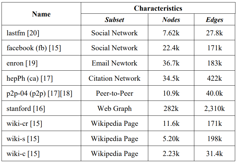
TABLE 1. REAL-WORLD GRAPHS FROM SNAP [6]

Once measured, Principal Component Analysis will be performed, and all the generated and real-world graphs will be plotted in a space consisting of the first principal component as the x-axis and the second principal component as the y-axis. Once graphed, it can be seen whether the generated graphs cover the set of selected real-world graphs.

This is a similar method when evaluating the coverage space of the SPEC benchmark suite. [11] However, a significant difference is that in this case, PCA explains variance in graph structure, whereas in Phansalkar, it explains variance in measured performance metrics. This leaves a gap that this article must address by showing that the placement of a graph in this PCA space relates to the final hardware performance. Each graph will be run on a suite of graph algorithm workloads. Then, for each graph, the correlation of the performance of these workloads to other graphs will be compared to the distance between the graphs. Once the correlation of performance is related to distance, a clustering algorithm can be run to reduce the set. In addition, if distance is shown to have a significant correlation to performance, one can use the distance between a real-world graph and the benchmark graphs to select a benchmark graph, making this method back-annotatable.

D. Significance of Euclidean Distance

These graphs were run on a benchmark suite, OpenGraph, which performs the following kernels [12]:

• PageRank: A way of measuring the importance of a specific node in a graph. Popular inside search engines.

• SSSP Delta and Belford: These are two methods of finding all shortest paths starting at a random node for each iteration.

• Depth First Search: A depth-first search from a specific vertex to a random vertex each iteration.

• SPMV: Sparse Matrix Multiply algorithm. An algorithm that helps multiply many vertices in a sparse graph.

• Connected Components: Labels connected graphs inside the given edge list.

• Betweenness: The betweenness centrality score of all vertices in the graph.

• Triangle Counting: Computes the total number of triangles in the graph

These benchmarks are derived from the GAP benchmark suite. [7] The overarching idea in selecting these kernels is that more extensive graph algorithms will consist mainly of these kernels; thus, the performance of these kernels will relate to more comprehensive programs.

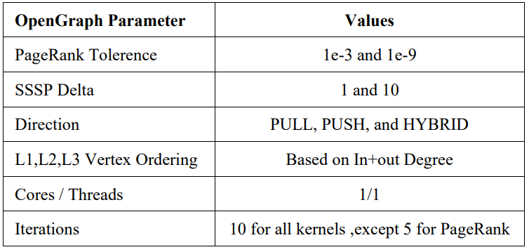
TABLE 2. OPENGRAPH BENCHMARK PARAMETERS

These benchmark workloads were run on an AWS m4.large EC2 instance with no other programs running. The hardware specs are as follows: Intel Xeon Haswell running at 2.4GHz, 2 Virtual CPUs, and 8GB of Memory running Ubuntu.

A total of 33 graph workloads were run on each generated graph, creating a performance profile for a graph that includes 33 runtimes. Next, an Ordinary Least Squared fit was run between each of the generated graphs, showing how the performance of one graph correlated with another through a calculated R2 value. Next, these R2 values were plotted against the Euclidean distance between the two graphs in the PCA space. The resulting plot will show how much the Euclidean distance between graphs in the PCA space correlates to how similar the hardware performance is between the graphs. Ideally, the smaller the distance, the higher the R2 score. Knowing this distance is significant, graphs can start being clustered based on the distance to group the graphs.

E. Graph Selection

Once the distance is deemed significant, k-means and hierarchical clustering are performed on the set of graphs. For k-means clustering, ten clusters were chosen based on visual analysis of the graph of the PCA space. Future work can explore how using more or less may be better in the long term.

The k-means clustering will group all graphs into ten clusters. The centroid is found for each cluster, and the graph closest to the centroid will represent that cluster. After this step, the original, more extensive group of about one hundred generated graphs is reduced to a smaller set of ten, which will be considered the final "Lambda Set" benchmark graphs.

Hierarchical clustering will also be performed to analyze how even the grouping of graphs is and to see if any graph is a significant outlier that should be included in the final benchmark. This will be analyzed at 25 clusters and below, as the full dendrogram is challenging to interpret without making some initial clusters. Hierarchical clustering is used mainly for analysis rather than picking resulting graphs.

F. Selection Evaluation

For the final step, the real-world graphs described in "C. Coverage Selection" will also run the same 33 graph workloads to get their performance profiles. The closest Lambda Set graph seen in the PCA space will be chosen to represent that real-world graph, and then the performance profile of that Lambda Set graph will be fit using Ordinary Least Squares to the performance profile of the real-world graph. The resulting R2 value will be used to evaluate how well each selected Lambda Set graph represents the matched real-world graph.

If the results are positive, the back-annotation property needed from the benchmark is also supported. To match a Lambda Set graph to a real-world graph or a real-world graph to a Lambda Set graph, all that has to be done is find the closest graph in the PCA space described above.

In addition, it can be used as a graph generator. For example, the closest lambda graph can be found if there is a real-world graph with 10 million nodes. Using the lambda value of that Lambda Set graph, one can use the complex graph generator to make a representative graph with a scaled-down number of nodes.

V. RESULTS

A. Complex Graph Generation

The complex graph generation had very similar results to the paper on which it was based. As lambda was swept from 0 to 1, the same structure was seen at each respective lambda point. A sampling of generated lambda graphs can be seen below.

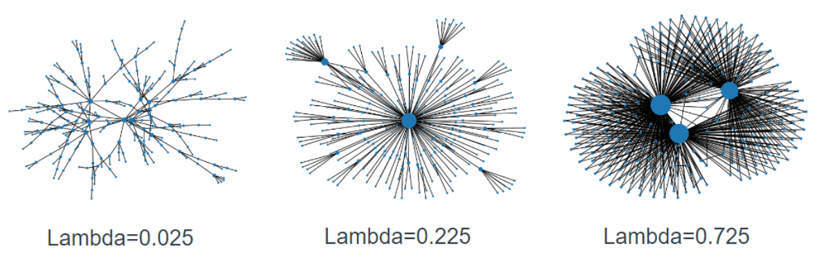
Figure A. Example Generated Graphs.

The graphs converged to a final p and d value and showed no oscillation in covering a final solution. Sometimes, the runs took a long time to optimize the last couple of edges in the original runs; however, the updated algorithm stopped the process and deemed it converged once the change reached a certain level.

B. Coverage Evaluation

The first two components of the PCA were found. The first component explained 79.83% of the variance in graph structure seen inside the generated graphs, and the second component explained 15.87% of the graph structure. These two components explain 95.7% of the variance in the structural properties seen in all the generated lambda graphs, which is a significant amount.

The first plot explored how the lambda value affected the placement of graphs in this PCA space. To do this, the first PCA component was placed on the x-axis and the second on the y-axis, and a color was assigned to each range of lambda values.

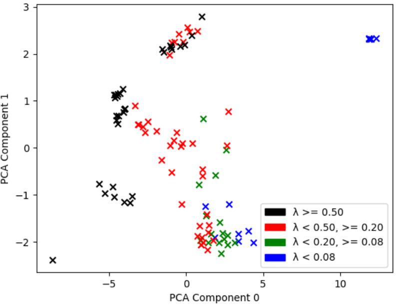
Figure 1. Generated Graphs in PCA Space with Respect to Lambda Ranges

Figure 1 above shows that as lambda is swept from 0 to 1, the generated graphs also sweep the PCA space. This can also be used in future work to highlight what lambda ranges might want lower resolution. For example, the gap in lambda graphs < 0.08 can point to the need for a higher resolution than 0.01. The same can be said for lambda graphs >= 0.50. However, the generated lambda graphs showed good space coverage.

Next, the real-world graphs were plotted in the same space as before. This time, all lambda graphs are blue, and all real-world graphs are red with the name as a label.

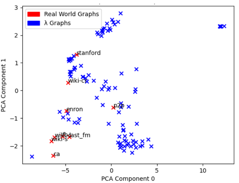
Figure 2. Real-World Graphs compared to Generated Graphs in PCA Space

Figure 2 shows the lambda graph space covers the selected real-world graphs relatively well. Again, we can use this for future work, as more real-world graphs should be selected for analysis that fit in the right portion of the graph. By intuition, this PCA space would be filled with more random, small-world graphs like roadways and subway systems. All sample SNAP graphs in this area were too large to analyze time-permitting. Overall, these results were also very positive.

C. Significance of Euclidean Distance

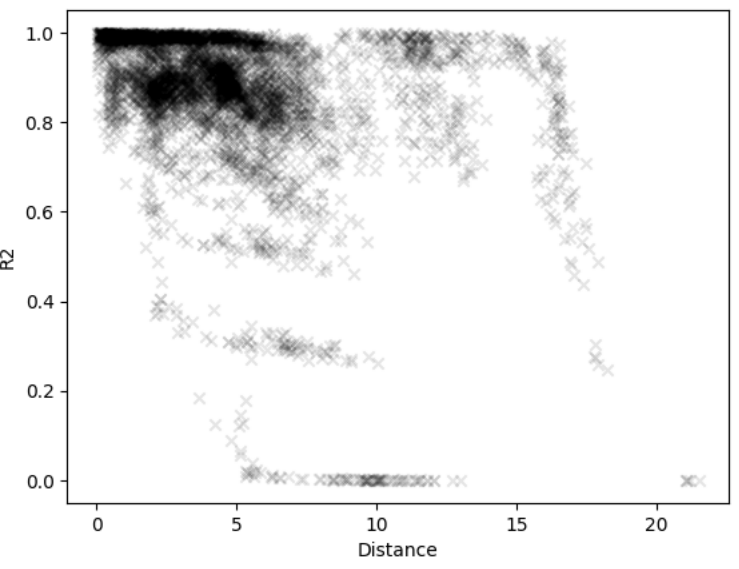
Figure 3. Linear Correlation of Performance verses Distance in PCA Space

After exploring the PCA space, the significance of distance was determined. First, the correlation between the two graphs (R2 value) was plotted against the Euclidean distance between them.

In these figures, the shorter distance between the two graphs resulted in a higher correlation in their performance profiles. After this, an OLS fit was done between distance and R2 value, which showed a significant coefficient with a t-value above 100.

D. Graph Selection

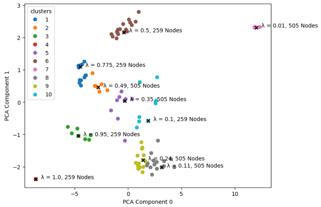
Figure 4 . k-Means Clustering and Selection of Final Ten Lambda Set Graphs

K-means clustering was then performed to create ten clusters, as shown in Figure 4 above. The resulting final set of graphs is the following (Lambda, Number of Nodes): (1.0,259), (0.11,505), (0.24,505), (0.95,259), (0.1,259), (0.35,505), (0.49,505), (0.775,259), (0.5,259), (0.01,505)

The figure shows that the selected graphs provide good coverage over the PCA space, meaning ten is a relatively good number of graphs representing this space.

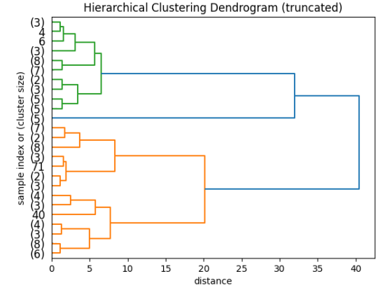
Figure 5. Dendrogram of Lambda Graph Hierarchical Clustering

Next, a dendrogram was constructed truncated at 25 clusters for easy analysis (Figure 5). This dendrogram shows how the clustering of graphs is relatively even, with groups staying around 4 to 8. This was mainly used to see how evenly spaced these clusters were in the PCA space, and how spread the selected benchmarks would be. In addition, future work could use (a full-sized) dendrogram to create larger or smaller sets than ten graphs. Overall, there were no actual outlier graphs, with the most significant outlier being a group of five graphs making it to the third level.

E. Selection Evaluation

One graph was selected to represent each real-world graph by finding the closest in the PCA space to evaluate this final set. Then, the performance profiles of the real-world graph and the chosen benchmark graph were compared using OLS. Figure 6 shows that for all of the graphs, there was a high correlation between the benchmark graph selected and the real-world graph. This indicates that the benchmark set does a good job explaining how these real-world graphs would perform on specific hardware platforms, with most of the R2 values being above 0.85 and having significant coefficients with t values above 10. (At least the hardware platform for this project was run on.)

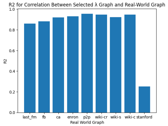
Figure 6. Performance Correlation of Selected Lambda Set Graph to Real-world Graph

The most extensive real-world graph, Stanford, did show a single negative result, so further analysis was done to see how the performance profiles differed. To do this, the runtimes of the benchmark graph were plotted against the runtimes of the Stanford graph, resulting in Figure 7 below.

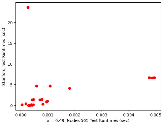
Figure 7. Workload runtime on Selected Graph verses stanford graph.

One outlier can be seen, which destroys the R2 value. However, the parameter was still significant. One interesting point is that each kernel is run three times. One was for the PUSH, PULL, and HYBRID approaches for processing the graph, meaning that two of the three were predictable approaches. However, one of the methods proved significantly less efficient to run. It could be assumed that the most efficient method would be chosen to run a kernel. However, that is a jump in logic that cannot be proved in this project's scope, so this data point stays.

Overall, the selected benchmark graphs provided high R2 correlation in almost all cases and significant coefficients in every case; using these selected graphs did a good job representing this real-world set. However, one downside is that many of the graphs chose the same Lambda Set graph since they were so close together. A wider variety of real-world graphs is needed to prove the concept. However, this further supports the initial motivation as it shows how difficult it can be to choose a set of representative real-world graphs by going through the SNAP database and selecting graphs in different categories.

VI. CONCLUSION / FUTURE WORK

A. Future Work

There is a lot of future work. The first priority would be moving all network creation to C/C++, not Python. This will allow for the generation of larger, complex graph sets. With the move to C/C++, more analysis can also be done on a wider variety and size of real-world graphs, which is needed to prove this idea. Also, creating small, medium, and large Lambda Sets with a specific range of node sizes. Further research can then be done into how well the set of lambda graphs of a particular size relates to real-world graphs of a specific size. For example, could the small set do a good job representing real-world graphs with 1 to 199k nodes, the medium with 199k to 5 million nodes, etc.

B. Conclusions

Going back to the characteristics stated at the start of the article:

• Simple: The complex graph generator is simple in that it has fewer steps and parameters compared to many of the recursive graph generators that are used today. Just by published paper length, many of the recursive generators are tens of pages, whereas this complex generator was a three-page paper. Since the generator is simple, understanding the benchmark graphs and knowing how they were selected and what they represent is also simple.

• Realistic: The PCA analysis showed that the generated graphs could contain similar structural characteristics to real-world graphs. In addition, comparing the performance of the final "Lambda Set" graphs to real-world graphs shows that this set is realistic in representing the hardware performance of real-world graphs.

• Parsimonious: The generator only has a single parameter, meaning that the set of generated graphs contains graphs representing the parameter lambda from 0 to 1. The number of nodes can also be considered a parameter. However, this is inescapable for any generator.

• Flexible: Through visual analysis, it was seen that the set of lambda graphs generated contains a wide variety of structures, and the PCA analysis further supports that the generated graphs explain over 95% of the structural space.

• Fast: This suite did fall short in terms of speed, in my opinion. However, these graphs only must be generated once and can be made in parallel. Ultimately, this generation will never scale linearly with edge count, a significant problem for future investigation.

• Back-Annotatable: Showing that the distance in this PCA space is significant, one can annotate a real-world graph to a "Lambda Set" graph using distance relatively quickly. In addition, once the benchmark graph is found, lambda can be used with the complex graph generator to make smaller representative graphs of that large real-world graph.

Overall, this project showed a methodology for producing a set of representative graphs that can be used to profile how the hardware would perform on various graphs it might see.

Thanks for taking the time to read about my latest project.

Download the Lambda Set Edgelist (And all other Graphs used) here: Link

VII. REFERENCES

[1] J. Zhou, G. Cui, Z. Zhang, C. Yang, Z. Liu, and M. Sun, "Graph Neural Networks: A Review of Methods and Applications," in CoRR, vol. abs/1812.08434, 2018. [Online].

[2] P. Mehrotra, V. Anand, D. Margo, M. R. Hajidehi, and M. Seltzer, "SoK: The Faults in our Graph Benchmarks," 2024. [Online]. Available: https://arxiv.org/abs/2404.00766

[3] L. Kelvin, "Electrical Units of Measurement," in Popular Lectures and Addresses, vol. 1, 1891, p. 73.

[4] R. Ferrer i Cancho and R. V. Sole, "Optimization in complex networks," 2001. [Online]. Available: https://arxiv.org/abs/cond-mat/0111222

[5] L. Akoglu and C. Faloutsos, "RTG: A Recursive Realistic Graph Generator Using Random Typing," in Machine Learning and Knowledge Discovery in Databases, W. Buntine, M. Grobelnik, D. Mladenić, and J. Shawe-Taylor, Eds. Berlin, Heidelberg: Springer Berlin Heidelberg, 2009, pp. 13-28.

[6] J. Leskovec and A. Krevl, "SNAP Datasets: Stanford Large Network Dataset Collection," [Online]. Available: http://snap.stanford.edu/data, Jun. 2014.

[7] S. Beamer, K. Asanović, and D. Patterson, "The GAP Benchmark Suite," 2017. [Online]. Available: https://arxiv.org/abs/1508.03619

[8] P. Erdős and A. Rényi, "On Random Graphs I," Publicationes Mathematicae Debrecen, 1959.

[9] D. J. Watts and S. H. Strogatz, "Collective dynamics of 'small-world' networks," Nature, vol. 393, no. 6684, pp. 440-442, 1998.

[10] A.-L. Barabási and R. Albert, "Emergence of Scaling in Random Networks," Science, vol. 286, no. 5439, pp. 509–512, Oct. 1999. [Online]. Available: http://dx.doi.org/10.1126/science.286.5439.509

[11] A. Phansalkar, A. M. Joshi, and L. K. John, "Analysis of redundancy and application balance in the SPEC CPU2006 benchmark suite," in International Symposium on Computer Architecture, 2007. [Online]. Available: https://api.semanticscholar.org/CorpusID:17651294

[12] A. Mughrabi, OpenGraph. (n.d.). Retrieved from https://github.com/atmughrabi/OpenGraph

[13] W. Hu, M. Fey, M. Zitnik, Y. Dong, H. Ren, B. Liu, M. Catasta, and J. Leskovec, "Open Graph Benchmark: Datasets for Machine Learning on Graphs," arXiv preprint arXiv:2005.00687, 2020.

[14] Aric A. Hagberg, Daniel A. Schult and Pieter J. Swart, "Exploring network structure, dynamics, and function using NetworkX", in Proceedings of the 7th Python in Science Conference (SciPy2008), Gäel Varoquaux, Travis Vaught, and Jarrod Millman (Eds), (Pasadena, CA USA), pp. 11–15, Aug 2008

[15] B. Rozemberczki, C. Allen, and R. Sarkar, "Multi-scale Attributed Node Embedding," arXiv preprint arXiv:1909.13021, 2019.

[16] J. Leskovec, K. Lang, A. Dasgupta, M. Mahoney. Community Structure in Large Networks: Natural Cluster Sizes and the Absence of Large WellDefined Clusters. Internet Mathematics 6(1) 29--123, 2009.

[17] J. Leskovec, J. Kleinberg and C. Faloutsos. Graph Evolution: Densification and Shrinking Diameters. ACM Transactions on Knowledge Discovery from Data (ACM TKDD), 1(1), 2007.

[18] M. Ripeanu and I. Foster and A. Iamnitchi. Mapping the Gnutella Network: Properties of Large-Scale Peer-to-Peer Systems and Implications for System Design. IEEE Internet Computing Journal, 2002.

[19] B. Klimmt, Y. Yang. Introducing the Enron corpus. CEAS conference, 2004.

[20] B. Rozemberczki and R. Sarkar, "Characteristic Functions on Graphs: Birds of a Feather, from Statistical Descriptors to Parametric Models," in Proceedings of the 29th ACM International Conference on Information and Knowledge Management (CIKM' 20), pp. 1325–1334, ACM, 2020.

[21] J. Palowitch, A. Tsitsulin, B. Mayer, and B. Perozzi, "GraphWorld: Fake Graphs Bring Real Insights for GNNs," in Proceedings of the 28th ACM SIGKDD Conference on Knowledge Discovery and Data Mining (KDD' 22), ACM, Aug. 2022. [Online]. Available: http://dx.doi.org/10.1145/3534678.3539203