Using Autoencoder Neural Nets to Compress and/or Upscale Video
One thing that always interested me about Machine Learning is that a computer, which seemingly runs by a strict set of rules, could create new things. So I started looking into the methods of how to do that and ran into Autoencoders. I thought something interesting to do would be to create an Autoencoder that could train on a video and learn to create intermediate frames. This could be a form of compression where one could remove half of the frames and instead package a Neural Net with the file to generate the intermediate frames. A video could also be upscaled to a higher fps using this method.
Both these things have been done before, and there are plenty of papers describing methods to achieve this. However, when I started reading the articles, I will not lie; a lot went over my head. Typically, what I like to do when academic papers aren't making much sense is approaching the problem as if no one has touched it before. Often, I gain a deeper understanding of the problem that is trying to be solved. When I read through the paper again, it's almost like you gain a context that explains why certain things are being said and the motivations behind different methods used.
So that is what I did here. I went through finding out how to create new frames based on surrounding frames and then made a guide on how to do some of the things I did. After the first half of this project was completed I went back through the papers saw clearly what mistakes I made, what could be added to the models to make them better, and how the paper solved the presented problems.
In this guide, we are going to cover topics including:
Exploring a basic Autoencoder Structure
Using Keras's Functional Model Builder to create a two-input model.
Exploring methods to measure output frame quality.
Exploring ways not to use up every ounce of RAM to load training data.
Using Keras's Functional Model to create more Complex Structures
The only prerequisite for you is a Gmail account where you set up Google Drive before (If you want to save your models and data). The tools we are going to use are:
Google Collab - Free Online Python Notebook. (Or any Python Environment)
Note: I used Collab Pro for extra RAM and training time.
Tensorflow Keras - Neural Net Building and Testing
cv2 - For Video Frame Extraction and mp4 Creation
This guide starts out with the assumption you can open up a new Google Collab notebook and Python knowledge. That's about it.
If you just want to look at the code, skip to Initial Frame Setup and Execution
Whats an Autoencoder and Why use it for this Application
For this application, we need to have the ability to make a Neural Net that takes in some information about two frames and constructs another frame. Autoencoder Architectures are perfect for this (and built for it).
These architectures consist of two main parts, the encoder, and the decoder. The encoder breaks down information into some smaller set, almost like breaking down a picture into what objects are in the picture. The decoder takes this smaller set of data to generate a more extensive set of information, for example, taking a list of objects and creating a picture from them.

From Chervinskii on Wikipedia
Autoencoders can be used in many applications such as Audio Generation, Picture Denoising, and Language Translation. But today, we will be wising them for frame generation.
Theory on How to Approach This
Our general problem is that we are trying to create a frame from two other frames. If we are trying to compress a file we need to remove some amount of frames and generate them at a later time using the Autoencoder. If we are trying to upscale, we are trying to create entirely new frames from the frames around it. This means our model's input needs to have information from two frames to create a single frame. Since I don't know how to make dual input neural nets (but we will learn later), I decided that the best start is to use the difference between frames as the input. Then the output will be the difference between the first and predicted frame.
So we need to follow the pattern:
Input : (Frame 2 - Frame 0), Output: (Frame 1 - Frame 0)
Input : (Frame 3 - Frame 1), Output: (Frame 2 - Frame 1)
…
To get a predicted frame we would have to do the following:
pred = frame0 + model.predict(frame2 - frame0)
This gives us a model that could take any two frames and predict a frame in between, and this allows us to compress or upscale video. Next, I ran into the question of "How we measure how good our model is?"
Ways to Measure Frame Quality
When I looked into how to measure frame quality, I ran into three main measures: PSNR, SSIM, and MSE. However, it ultimately came down to the fact that there is no perfect measure. What the eye sees as "good" video is complex and not very measurable or tangible. Netflix on their tech blog had a good article on this (https://netflixtechblog.com/toward-a-practical-perceptual-video-quality-metric-653f208b9652) showing how they approached measuring video quality.
MSE (Mean Squared Error): This is the metric the model will use for the error calculation. However, it is a relatively bad overall heuristic of how good a model performs. For example, if every pixel were “1” off, the picture would look brighter. However, a frame with half of the pixels “1” off would look noisy but have a smaller MSE. So we should have other metrics we look at to make sure our model is genuinely making progress while learning.
PSNR (Peak Signal to Noise Ratio): The signal-to-noise ratio tries to measure the actual proportion of noise to the maximum possible value of a pixel rather than just the difference between the predicted and actual. This is on a logarithmic scale so minor differences won't factor in as much, and the final number mostly is how far off-peak differences are.

Todd Veldhuizen:
https://homepages.inf.ed.ac.uk/rbf/CVonline/LOCAL_COPIES/VELDHUIZEN/node18.html
SSIM (Structural Similarity Index Measure): This measure is more complex, and I haven’t heard about it before this project. I would recommend looking more into it outside this post. However, it tries to take into account differences in luminance, contrast, and structure. I found the SSIM to be the most reliable in measuring how well a model performs. Below shows an example of pictures with the same PSNR but improving SSIM.

https://medium.com/@datamonsters/
Later on, we will actually see our best model actually has a higher MSE (bad), but a higher PSNR and SSIM (good).
Initial Setup and Frame Extraction
One disclaimer is that I used Google Colab Pro as I kept running out of memory for the frames. Below I show a method in which you don't need high memory nodes. At that point, the only benefit of pro is doing long training runs without timing out the worksheet.
Before we start making a model, lets:
Install/Import our packages
Create Functions to Measure Frame Quality
Create Helper Function to Fit Model
Extract Model Parameters and Frames from Video
Look at some of the frames
Install and Import Packages
import matplotlib.pyplot as plt
import numpy as np
import pandas as pd
import tensorflow as tf
import larq as lq
import seaborn as sns; sns.set_theme()

from sklearn.metrics import accuracy_score, precision_score, recall_score
from sklearn.model_selection import train_test_split
from tensorflow.keras import layers, losses
from tensorflow.keras.datasets import fashion_mnist
from tensorflow.keras.models import Model
from tensorflow import keras
from google.colab import drive
from google.colab import files
from google.colab.patches import cv2_imshow

from keras import backend as K

import cv2
plt.rcParams["axes.grid"] = False

# In Collab we are going to use GPUs so we just want tes test that tensfor flow is connected up top a GPU.
%tensorflow_version 2.x
import tensorflow as tf
device_name = tf.test.gpu_device_name()
if device_name != '/device:GPU:0':
  raise SystemError('GPU device not found')
print('Found GPU at: {}'.format(device_name))

from psutil import virtual_memory
ram_gb = virtual_memory().total / 1e9
print('Your runtime has {:.1f} gigabytes of available RAM\n'.format(ram_gb))

# Since we are going to be reading alot of frames we need to make sure we are on a high-ram instance.
if ram_gb < 20:
  print('To enable a high-RAM runtime, select the Runtime > "Change runtime type"')
  print('menu, and then select High-RAM in the Runtime shape dropdown. Then, ')
  print('re-execute this cell.')
else:
  print('You are using a high-RAM runtime!')

# We are going to want to save our models, data, and diagrams as we go through the project.
google_drive_path = "/content/drive/My Drive/Project_2/"
from google.colab import drive
drive.mount('/content/drive')
Create Functions to Measure Frame Quality
# Calculate PSNR from two frames
def PSNR(y_true, y_pred):
    max_pixel = 1.0
    return (10.0 * K.log((max_pixel ** 2) / (K.mean(K.square(y_pred - y_true), axis=-1))))

# Create a wrapper function around the Tensorflow function.
def SSIM(y_true, y_pred):
    return tf.image.ssim(y_true,y_pred,max_val=1)
Create Helper Function to Fit Model
# Method defining how an iteration on a model is run. Returns historical training statistics.
# This makes the training loops cleaner.
def run_model_iteration( model, x_train_np, y_train_np, epochs, batch_size) :
  hist = model.fit(x_train_np, y_train_np,
                  epochs=epochs,
                  shuffle=True,
                  batch_size=batch_size,
                  validation_split=0.2)

  # Function assumes the PSNR and SSIM metrics are added to the model when compiled.
  toReturn = dict();
  toReturn['loss'] = hist.history['loss']
  toReturn['PSNR'] = hist.history['PSNR']
  toReturn['SSIM'] = hist.history['SSIM']

  return toReturn
Extract Model Parameters and Frames from Video
#Extract Frames from the video and get essential information
vidcap = cv2.VideoCapture(google_drive_path + 'traffic_sd.mp4')
success,image = vidcap.read()
count = 0
height = 0
width = 0
channels = 0
fps = 0

fps = vidcap.get(cv2.CAP_PROP_FPS)
while success:
  cv2.imwrite(google_drive_path + "out_frame/frame%d.jpg" % count, image)     # save frame as JPEG file
  print(count)
  success,image = vidcap.read()
  # Just capture info on the first frame read
  if ( count == 1 ):
    height, width, channels = image.shape
  count += 1

print(height, width, channels, fps)

> 360 640 3 25.0
Look at some of the frames
# Grab some Images
img0 = cv2.imread(google_drive_path + "out_frame/frame%d.jpg" % 3)         # save frame as JPEG file
img1 = cv2.imread(google_drive_path + "out_frame/frame%d.jpg" % (3+1))     # save frame as JPEG file
img2 = cv2.imread(google_drive_path + "out_frame/frame%d.jpg" % (3+2))     # save frame as JPEG file

# Differance Accors Two Frames
into = (img2/255) - (img0/255)
# Differance Accross the One Frame
outof = (img1/255) - (img0/255)

plt.imshow(into)
plt.show()  # display it
Autoencoder
Now that we have our data, we need to create a training loop that will process the data in chunks:
Create Autoencoder using Keras Sequential Model
Setup the Optimizer and Compile
Create loop which loads partial data, trains model, and stores results.
Graph the Training History
Visualize the Results
Create Autoencoder using Keras Sequential Model
The way we define an Autoencoder using a sequential model is defining two separate models:
The encoder consisting of an Input Layer and Convolutional Layers reducing dimensionality.
And the decoder increasing the dimensionality of the output of the encoder.
The final model essentially combines these two models into one single model.
Just to note the model does not have to be this way but gives a nice separation between the encoder and decoder.
Since all the values are differences between two frames their values can range from [-1,1]. This is why I used the ‘tanh’ activation function as it has close to the same range. (-1,1).
# Create Auto Encoder Model
class VideoModel(Model):
  def __init__(self):
    super(VideoModel, self).__init__()
    self.encoder = tf.keras.Sequential([
      layers.Input(shape=(height, width, channels)),
      layers.Conv2D(240, (3,3), activation='tanh', padding='same', strides=2),
      layers.Conv2D(64, (3,3), activation='tanh', padding='same', strides=2),
      layers.Conv2D(16, (3,3), activation='tanh', padding='same', strides=2)])

    self.decoder = tf.keras.Sequential([
      layers.Conv2DTranspose(16, kernel_size=3, strides=2, activation='tanh', padding='same'),
      layers.Conv2DTranspose(64, kernel_size=3, strides=2, activation='tanh', padding='same'),
      layers.Conv2DTranspose(240, kernel_size=3, strides=2, activation='tanh', padding='same'),
      layers.Conv2D(3, kernel_size=(3,3), activation='tanh', padding='same')])

  def call(self, x):
    encoded = self.encoder(x)
    decoded = self.decoder(encoded)
    return decoded

autoencoder = VideoModel()
Setup the Optimizer and Compile
For the optimizer, I used Adam with configurations very similar to what I used in a previous image processing project for a class as the previous project worked with similar resolution pictures. This would be a good place to hypertune the model, however, I was lazy and just used values straight from a previous project.
Then we compile adding our PSNR and SSIM metrics to the model.
# initiate Adam optimizer
opt = tf.keras.optimizers.Adam(learning_rate=0.0001, beta_1=0.9, beta_2=0.999, epsilon=1e-08)
autoencoder.compile( optimizer=opt, metrics=[PSNR, SSIM], loss=losses.MeanSquaredError())
Create loop which loads partial data, trains model, and stores results.
At first, I used HD Video data which crashed my Google Collab space many times over. To combat this, we have to bring the frames in chunk by chunk to train the model.
The loop grabs a chunk of frames, then looping through that chunk of frames, populates the x and y training sets with the appropriate processed frames. We are operating on the differences for this model, so we need to do a subtraction first. Once the training sets for that chunk are complete, the data is put into the model for fitting.
We also have to set up a structure that will store all the training histories that are returned for each chunk to analyze them later.
# How many blocks of data to process.
block_amount = 10
# How many frames per block of data.
block_size = 50

hist_loss = []
hist_psnr = []
hist_ssim = []

for block in range(0,block_amount) :
  # Create X and Y Train Arrays
  x_train = []
  y_train = []

  print("Loading Block: " , block)
  for i in range(0,block_size) :

    # Grab Frame 0,1,2
    print("Grabbing Frame: " , ((block_size * block) + i) )
    img0 = cv2.imread(google_drive_path + "out_frame/frame%d.jpg" % ((block_size * block) + i))
    img1 = cv2.imread(google_drive_path + "out_frame/frame%d.jpg" % ((block_size * block) + (i+1)))
    img2 = cv2.imread(google_drive_path + "out_frame/frame%d.jpg" % ((block_size * block) + (i+2)))

    # We want to train the model to predict differance to the next frame from the differance of the 0 and 2 frames
    x_train.append((img2/255) - (img0/255))
    y_train.append((img1/255) - (img0/255))

  print("Loaded Block: " , block)
  x_train_np = np.array(x_train)
  y_train_np = np.array(y_train)

  # Fit model over block of data and store history
  historyObj = run_model_iteration(
      autoencoder,
      x_train_np,
      y_train_np,
      512,
      4
      )
  print("Trained Block: " , block)

  hist_loss = hist_loss + historyObj['loss']
  hist_psnr = hist_psnr + historyObj['PSNR']
  hist_ssim = hist_ssim + historyObj['SSIM']

np.save(google_drive_path+"hist_loss" , hist_loss)
np.save(google_drive_path+"hist_psnr" , hist_psnr)
np.save(google_drive_path+"hist_ssim" , hist_ssim)
Graph the Training History
Using a simple plot, we can see the progress the model made chunk by chunk. Generally, I used this when deciding how many epochs the model should run. I tried to get close to when each chunk converged on a value. However, I didn’t want to overtrain to any specific chunk (and overall, the run had to finish before Google Collab timed out.)
# plot Loss
plt.plot(hist_loss, label='test')
plt.savefig(google_drive_path+ "one_input_model_loss.png")
plt.legend()
plt.show()

One Input Autoencoder Loss
# plot PSNR
plt.plot(hist_psnr, label='PSNR')
plt.savefig(google_drive_path+ "one_input_model_PSNR.png")
plt.legend()
plt.show()

One Input Autoencoder PSNR
# plot SSIM
plt.plot(hist_ssim, label='SSIM')
plt.savefig(google_drive_path+ "one_input_model_SSIM.png")
plt.legend()
plt.show()

One Input Autoencoder SSIM
From these, we can see there are definitely chunks of frames that are more difficult to predict than others. The loss seems to still have room to improve, however, our other metrics seemed to level out more.
Visualize the Results
To help visualize truly what is happening and how close the model is I used heatmaps to visualize the differences in the frames. So here we:
Make a heatmap of the actual differences.
Make a heatmap of the predicted differences
Make a heatmap of the difference between actual and predicted.
Each picture is a color channel of the image. (Red, Blue, Green)

For reference the first frame.
b_act,g_act,r_act = cv2.split(y_train_np[20])
fig, axs = plt.subplots(ncols=3,figsize=(100,20))
sns.heatmap(r_act, ax=axs[0], vmin=-1, vmax=1)
sns.heatmap(g_act, ax=axs[1], vmin=-1, vmax=1)
sns.heatmap(b_act, ax=axs[2], vmin=-1, vmax=1)

Actual Difference
diff = autoencoder.predict(np.array([x_train_np[20]]))
diff[0]
b_pred,g_pred,r_pred = cv2.split(diff[0])
fig, axs = plt.subplots(ncols=3,figsize=(100,20))
sns.heatmap(r_pred, ax=axs[0], vmin=-1, vmax=1)
sns.heatmap(g_pred, ax=axs[1], vmin=-1, vmax=1)
sns.heatmap(b_pred, ax=axs[2], vmin=-1, vmax=1)

Predicted Difference
r_amp = r_act - r_pred
g_amp = g_act - g_pred
b_amp = b_act - b_pred

fig, axs = plt.subplots(ncols=3,figsize=(100,20))
sns.heatmap(r_amp, ax=axs[0], vmin=-1, vmax=1)
sns.heatmap(g_amp, ax=axs[1], vmin=-1, vmax=1)
sns.heatmap(b_amp, ax=axs[2], vmin=-1, vmax=1)

Difference between predicted and actual.
Here we see the model does a relatively good job for the lighter moving areas, but for the fast-moving car on the left, it has trouble predicting. I think this is ok as long as it keeps a blur as its hard to differentiate between the “correct” blur someone would see.
Two Input Autoencoder
After I created the single input Autoencoder, I started thinking that there is possibly a better nonlinear way of combining the frames than a difference. To do this we need to make a two-input Autoencoder where both end frames are inputs, and the middle frame is the output with no extra processing.
Let's now try to create a multi-input model. We need to use the Keras Functional model to produce the Neural Net:
Create Autoencoder using Keras Functional Model
Setup the Optimizer and Compile
Create loop which loads partial data, trains model, and stores results.
Graph the Training History
Visualize the Results
Create Autoencoder using Keras Functional Model
For a two-input autoencoder, we now need to go away from the sequential model and move toward a functional model.
First, we need to create the encoder for both of our frames. This is very similar to above but just duplicated.
Second, we need to combine the encoded values from both encoders.
Finally, we need to decode the combined encoded values.
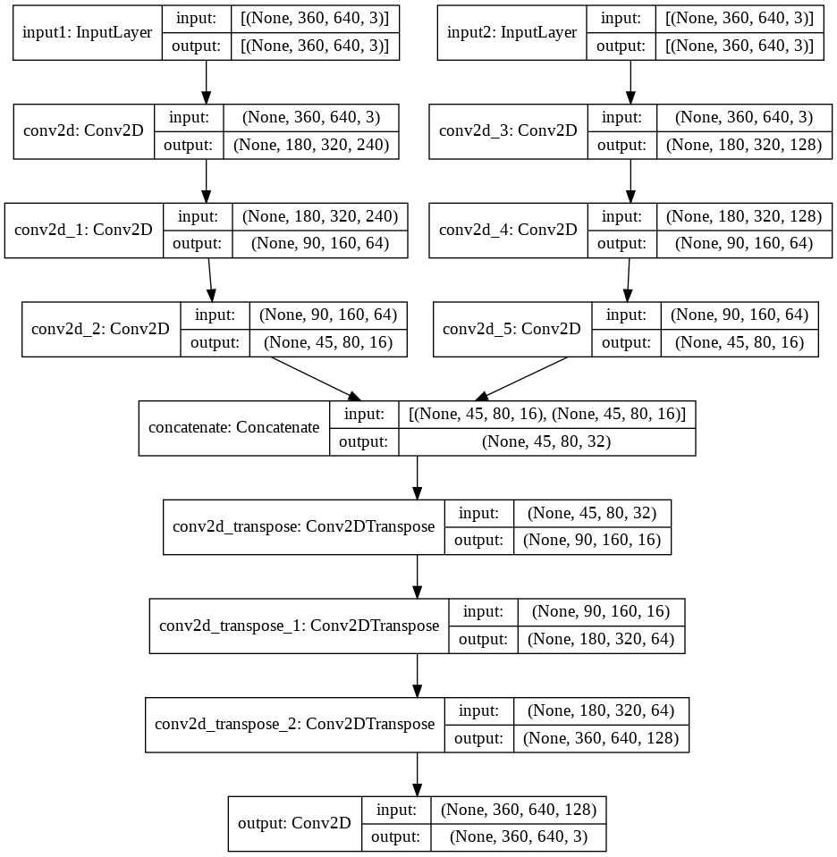
The functional model is very similar to the sequential model with the exception that each layer has to be stored in a variable and explicitly passed to the input of the next layer. This is what allows us to concatenate as we have references to two layers, whereas for a sequential model we only have access to the output of the previous layer.
Here we use ’relu’ because the inputs are now full frames and not the difference. This means that the values are only [0,1].
frame_0_input  = layers.Input(shape=(height, width, channels), name="input1");
x              = layers.Conv2D(240, (3,3), activation='relu', padding='same', strides=2)(frame_0_input)
x              = layers.Conv2D(64, (3,3), activation='relu', padding='same', strides=2)(x)
frame_0_output = layers.Conv2D(16, (3,3), activation='relu', padding='same', strides=2)(x)

frame_1_input  = keras.Input(shape=(height, width, channels), name="input2");
x              = layers.Conv2D(128, (3,3), activation='relu', padding='same', strides=2)(frame_1_input)
x              = layers.Conv2D(64, (3,3), activation='relu', padding='same', strides=2)(x)
frame_1_output = layers.Conv2D(16, (3,3), activation='relu', padding='same', strides=2)(x)

x = layers.concatenate([frame_0_output,frame_1_output])

x = layers.Conv2DTranspose(16, kernel_size=3, strides=2, activation='relu', padding='same')(x)
x = layers.Conv2DTranspose(64, kernel_size=3, strides=2, activation='relu', padding='same')(x)
x = layers.Conv2DTranspose(128, kernel_size=3, strides=2, activation='relu', padding='same')(x)
frame_0_output = layers.Conv2D(3, kernel_size=(3,3), activation='relu', padding='same', name="output")(x)

two_input_autoencoder = keras.Model(
    inputs=[frame_0_input, frame_1_input],
    outputs=[frame_0_output],
)

keras.utils.plot_model(two_input_autoencoder, google_drive_path+ "multi_input_autoencoder.png", show_shapes=True)
Setup the Optimizer and Compile
Same as the single output autoencoder.
# initiate Adam optimizer
opt = tf.keras.optimizers.Adam(learning_rate=0.0001, beta_1=0.9, beta_2=0.999, epsilon=1e-08)
two_input_autoencoder.compile( optimizer=opt, metrics=[PSNR,SSIM], loss=losses.MeanSquaredError())
Create loop which loads partial data, trains model, and stores results.
Same as before with the exception that full frames are now the training data and not the differences, so no subtraction is needed in this case. Only the division to get the data from 0 to 1.
block_amount = 10
block_size = 50

two_hist_loss = []
two_hist_psnr = []
two_hist_ssim = []

for block in range(0,block_amount) :
  # Create X and Y Train Arrays
  x_train_0 = []
  x_train_1 = []
  y_train = []

  print("Loading Block: " , block)
  for i in range(0,block_size) :

    # Grab Frame 0,1,2
    print("Grabbing Frame: " , ((block_size * block) + i) )
    img0 = cv2.imread(google_drive_path + "out_frame/frame%d.jpg" % ((block_size * block) + i))
    img1 = cv2.imread(google_drive_path + "out_frame/frame%d.jpg" % ((block_size * block) + (i+1)))
    img2 = cv2.imread(google_drive_path + "out_frame/frame%d.jpg" % ((block_size * block) + (i+2)))

    x_train_0.append((img0/255))
    x_train_1.append((img2/255))
    y_train.append((img1/255))

  print("Loaded Block: " , block)
  x_train_0_np = np.array(x_train_0)
  x_train_1_np = np.array(x_train_1)
  y_train_np = np.array(y_train)

  historyObj = run_model_iteration(two_input_autoencoder,
                                   {"input1": x_train_0_np, "input2" : x_train_1_np},
                                   y_train_np,
                                   512,
                                   4)
  print("Trained Block: " , block)

  two_hist_loss = two_hist_loss + historyObj['loss']
  two_hist_psnr = two_hist_psnr + historyObj['PSNR']
  two_hist_ssim = two_hist_ssim + historyObj['SSIM']

np.save(google_drive_path+"two_hist_loss" , two_hist_loss)
np.save(google_drive_path+"two_hist_psnr" , two_hist_psnr)
np.save(google_drive_path+"two_hist_ssim" , two_hist_ssim)

two_input_autoencoder.save_weights(google_drive_path+ "model/two_input_model.h5", overwrite=True)
Graph the Training History
Plots are the same as before, however here we want to compare against the single input Autoencoder case.
hist_loss = np.load(google_drive_path+"hist_loss.npy")
two_hist_loss = np.load(google_drive_path+"two_hist_loss.npy")

# plot loss
fig, ax1 = plt.subplots()

ax1.plot(two_hist_loss, label='loss', color='tab:red')
ax2 = ax1.twiny()
ax2.plot(hist_loss, label='loss', color='tab:blue')

plt.savefig(google_drive_path+ "two_input_model_loss.png")
plt.show()

Blue - Single Input , Red - Two Input
hist_psnr = np.load(google_drive_path+"hist_psnr.npy")
two_hist_psnr = np.load(google_drive_path+"two_hist_psnr.npy")

# plot psnr
fig, ax1 = plt.subplots()

ax1.plot(two_hist_psnr, label='psnr', color='tab:red')
ax2 = ax1.twiny()
ax2.plot(hist_psnr, label='psnr', color='tab:blue')

plt.savefig(google_drive_path+ "two_input_model_psnr.png")
plt.show()
Here there were many epochs where the PSNR was inf. This means there are missing data points when graphed so the use of this plot is limited.

Blue - Single Input , Red - Two Input
hist_ssim = np.load(google_drive_path+"hist_ssim.npy")
two_hist_ssim = np.load(google_drive_path+"two_hist_ssim.npy")

# plot ssim
fig, ax1 = plt.subplots()

ax1.plot(two_hist_ssim, label='ssim', color='tab:red')
ax2 = ax1.twiny()
ax2.plot(hist_ssim, label='ssim', color='tab:blue')


plt.savefig(google_drive_path+ "two_input_model_ssim.png")
plt.show()

Blue - Single Input , Red - Two Input
Here we see that the SSIM has greatly improved over the single input model. From my experience with this project, SSIM was a much more important factor than PSNR. I would say that the two input Autoencoder definitely had the advantage.
Visualize the Results
pred = two_input_autoencoder.predict(  {
                                        "input1" : np.array([x_train_0_np[15]]),
                                        "input2" : np.array([x_train_1_np[15]])
                                        }
                                      )

plt.imshow(pred[0])
plt.show()  # display it

Predicted Frame
plt.imshow(y_train[15])
plt.show()  # display it

Actual Frame
When looking at both the generated pictures we can see the predicted value has more of a blur to it. In addition, the moving car looks otherworldy, however, I would say this again is less important as the car is moving faster.
pred = two_input_autoencoder.predict(  {
                                        "input1" : np.array([x_train_0_np[15]]),
                                        "input2" : np.array([x_train_1_np[15]])
                                        }
                                      )

b_pred,g_pred,r_pred = cv2.split((pred[0] - y_train[14]))
fig, axs = plt.subplots(ncols=3,figsize=(100,20))
sns.heatmap(r_pred, ax=axs[0], vmin=-1, vmax=1)
sns.heatmap(g_pred, ax=axs[1], vmin=-1, vmax=1)
sns.heatmap(b_pred, ax=axs[2], vmin=-1, vmax=1)

Predicted
b_act,g_act,r_act = cv2.split(y_train[15] - y_train[14])
fig, axs = plt.subplots(ncols=3,figsize=(100,20))
sns.heatmap(r_act, ax=axs[0], vmin=-1, vmax=1)
sns.heatmap(g_act, ax=axs[1], vmin=-1, vmax=1)
sns.heatmap(b_act, ax=axs[2], vmin=-1, vmax=1)

Actual
r_amp = r_act - r_pred
g_amp = g_act - g_pred
b_amp = b_act - b_pred

fig, axs = plt.subplots(ncols=3,figsize=(100,20))
sns.heatmap(r_amp, ax=axs[0], vmin=-1, vmax=1)
sns.heatmap(g_amp, ax=axs[1], vmin=-1, vmax=1)
sns.heatmap(b_amp, ax=axs[2], vmin=-1, vmax=1)

Difference between Predicted and Actual
One interesting thing to note here is the front of the bus has an unusual difference spot to it, however, we can see there are very similar issues as before. One exception is that the predicted difference values are greater which leads to a sharper frame from what I have seen in this project.,.
One Input Autoencoder w/ Skip Paths
After I did the above experiments (and also experimented with some Quantized versions which didn’t work out) I revisited the paper to see what I may be missing. One major thing I saw in common in a lot of papers was the idea of skip layers. You need to use the Keras functional model to implement skip layers so I wase’t exactly sure how to implement them before, but now we do.
Skip layers take data from one level of an encoder and concatenate that layer to the corresponding decode layer.
So let's try to add the skip path to our one input Autoencoder
Create Autoencoder using Keras Functional Model
Setup the Optimizer and Compile
Create loop which loads partial data, trains model, and stores results.
Graph the Training History
Visualize the Results
Create Autoencoder using Keras Functional Model
Here we want to remake our single input sequential model into a functional model, and then we want to concatenate in previous layers of the encoder into the decoder. Below shows a diagram that better illustrates what the skip layers are doing.
frame_0_input  = keras.Input(shape=(height, width, channels), name="input2");
x1  = layers.Conv2D(128, (3,3), activation='tanh', padding='same', strides=2)(frame_0_input)
x2  = layers.Conv2D(64, (3,3), activation='tanh', padding='same', strides=2)(x1)
x3  = layers.Conv2D(16, (3,3), activation='tanh', padding='same', strides=2)(x2)
x4  = layers.Conv2DTranspose(16, kernel_size=3, strides=2, activation='tanh', padding='same')(x3)
sx4 = layers.concatenate([x4,x2])
x5  = layers.Conv2DTranspose(64, kernel_size=3, strides=2, activation='tanh', padding='same')(sx4)
sx5 = layers.concatenate([x5,x1])
x6  = layers.Conv2DTranspose(128, kernel_size=3, strides=2, activation='tanh', padding='same')(sx5)
frame_0_output = layers.Conv2D(3, kernel_size=(3,3), activation='tanh', padding='same', name="output")(x6)

skip_autoencoder = keras.Model(
    inputs=[frame_0_input],
    outputs=[frame_0_output]
)

keras.utils.plot_model(skip_autoencoder, google_drive_path+ "skip_autoencoder.png", show_shapes=True)

Setup the Optimizer and Compile
Same as before
# initiate Adam optimizer
opt = tf.keras.optimizers.Adam(0.00007, beta_1=0.9, beta_2=0.999, epsilon=1e-08)
skip_autoencoder.compile( optimizer=opt, metrics=[PSNR,SSIM], loss=losses.MeanAbsoluteError())
Create loop which loads partial data, trains model, and stores results.
Same as before (For Single Input Model)
block_amount = 10
block_size = 50

hist_loss = []
hist_psnr = []
hist_ssim = []

for block in range(0,block_amount) :
  # Create X and Y Train Arrays
  x_train = []
  y_train = []

  print("Loading Block: " , block)
  for i in range(0,block_size) :

    # Grab Frame 0,1,2
    print("Grabbing Frame: " , ((block_size * block) + i) )
    img0 = cv2.imread(google_drive_path + "out_frame/frame%d.jpg" % ((block_size * block) + i))
    img1 = cv2.imread(google_drive_path + "out_frame/frame%d.jpg" % ((block_size * block) + (i+1)))
    img2 = cv2.imread(google_drive_path + "out_frame/frame%d.jpg" % ((block_size * block) + (i+2)))

    # We want to train the model to predict differance to the next frame from the differance of the 0 and 2 frames
    x_train.append((img2/255) - (img0/255))
    y_train.append((img1/255) - (img0/255))

  print("Loaded Block: " , block)
  x_train_np = np.array(x_train)
  y_train_np = np.array(y_train)

  historyObj = run_model_iteration(
      skip_autoencoder,
      x_train_np,
      y_train_np,
      512,
      8
      )
  print("Trained Block: " , block)

  hist_loss = hist_loss + historyObj['loss']
  hist_psnr = hist_psnr + historyObj['PSNR']
  hist_ssim = hist_ssim + historyObj['SSIM']

np.save(google_drive_path+"hist_loss_skip" , hist_loss)
np.save(google_drive_path+"hist_psnr_skip" , hist_psnr)
np.save(google_drive_path+"hist_ssim_skip" , hist_ssim)

skip_autoencoder.save_weights(google_drive_path+ "model/model_skip.h5", overwrite=True)
Graph the Training History
Now lets compare how the skip version of the model did against the non-skip version.
hist_loss = np.load(google_drive_path+"hist_loss.npy")
hist_loss_skip = np.load(google_drive_path+"hist_loss_skip.npy")

# plot training history
fig, ax1 = plt.subplots()

ax1.plot(hist_loss, label='PSNR', color='tab:blue')
ax2 = ax1.twiny()
ax2.plot(hist_loss_skip, label='PSNR', color='tab:red')

plt.savefig(google_drive_path+ "skip_loss.png")
plt.show()

Red - Skip Version, Blue - Non-Skip Version
hist_psnr = np.load(google_drive_path+"hist_psnr.npy")
hist_psnr_skip = np.load(google_drive_path+"hist_psnr_skip.npy")

# plot training history
fig, ax1 = plt.subplots()

ax1.plot(hist_psnr, label='PSNR', color='tab:blue')
ax2 = ax1.twiny()
ax2.plot(hist_psnr_skip, label='PSNR', color='tab:red')

plt.savefig(google_drive_path+ "skip_psnr.png")
plt.show()

Red - Skip Version, Blue - Non-Skip Version
hist_ssim = np.load(google_drive_path+"hist_ssim.npy")
hist_ssim_skip = np.load(google_drive_path+"hist_ssim_skip.npy")

# plot training history
fig, ax1 = plt.subplots()

ax1.plot(hist_ssim, label='ssim', color='tab:blue')
ax2 = ax1.twiny()
ax2.plot(hist_ssim_skip, label='ssim', color='tab:red')

plt.savefig(google_drive_path+ "skip_ssim.png")
plt.show()

Red - Skip Version, Blue - Non-Skip Version
While the skip version had a worse loss, it had a lot better PSNR and SSIM.
Visualize the Results
Same as before.
x_train_0 = []
x_train_1 = []
y_train = []

for i in range(0,30) :
  # Grab Frame 0,1,2
  img0 = cv2.imread(google_drive_path + "out_frame/frame%d.jpg" % + i)
  img1 = cv2.imread(google_drive_path + "out_frame/frame%d.jpg" % + (i+1))
  img2 = cv2.imread(google_drive_path + "out_frame/frame%d.jpg" % + (i+2))

  # We want to train the model to predict differance to the next frame from the differance of the 0 and 2 frames
  x_train_0.append((img0/255))
  x_train_1.append((img2/255))
  y_train.append((img1/255))

x_train_0_np = np.array(x_train_0)
x_train_1_np = np.array(x_train_1)
y_train_np = np.array(y_train)
diff = skip_autoencoder.predict(np.array([x_train_np[20]]))
diff[0]
b_pred,g_pred,r_pred = cv2.split(diff[0])
fig, axs = plt.subplots(ncols=3,figsize=(100,20))
sns.heatmap(r_pred, ax=axs[0], vmin=-1, vmax=1)
sns.heatmap(g_pred, ax=axs[1], vmin=-1, vmax=1)
sns.heatmap(b_pred, ax=axs[2], vmin=-1, vmax=1)

Predicted
b_act,g_act,r_act = cv2.split(y_train_np[20])
fig, axs = plt.subplots(ncols=3,figsize=(100,20))
sns.heatmap(r_act, ax=axs[0], vmin=-1, vmax=1)
sns.heatmap(g_act, ax=axs[1], vmin=-1, vmax=1)
sns.heatmap(b_act, ax=axs[2], vmin=-1, vmax=1)

Actual
r_amp = r_act - r_pred
g_amp = g_act - g_pred
b_amp = b_act - b_pred

fig, axs = plt.subplots(ncols=3,figsize=(100,20))
sns.heatmap(r_amp, ax=axs[0], vmin=-1, vmax=1)
sns.heatmap(g_amp, ax=axs[1], vmin=-1, vmax=1)
sns.heatmap(b_amp, ax=axs[2], vmin=-1, vmax=1)

Difference between Predicted and Actual
Just by eyesight here we can see the model does a lot better job. Even with the person and car to the left, we see that the model is mostly missing sharpness rather than looking like an unrecognizable blur. This is something common I saw, neural nets have a lot of trouble in getting the sharpness of movement and a lot of the times suffer a blur effect.
Two Input Autoencoder w/ Skip Paths
Then let's try to add the skip path to our two input Autoencoder
Create Autoencoder using Keras Functional Model
Setup the Optimizer and Compile
Create loop which loads partial data, trains model, and stores results.
Graph the Training History
Visualize the Results
Create Autoencoder using Keras Functional Model
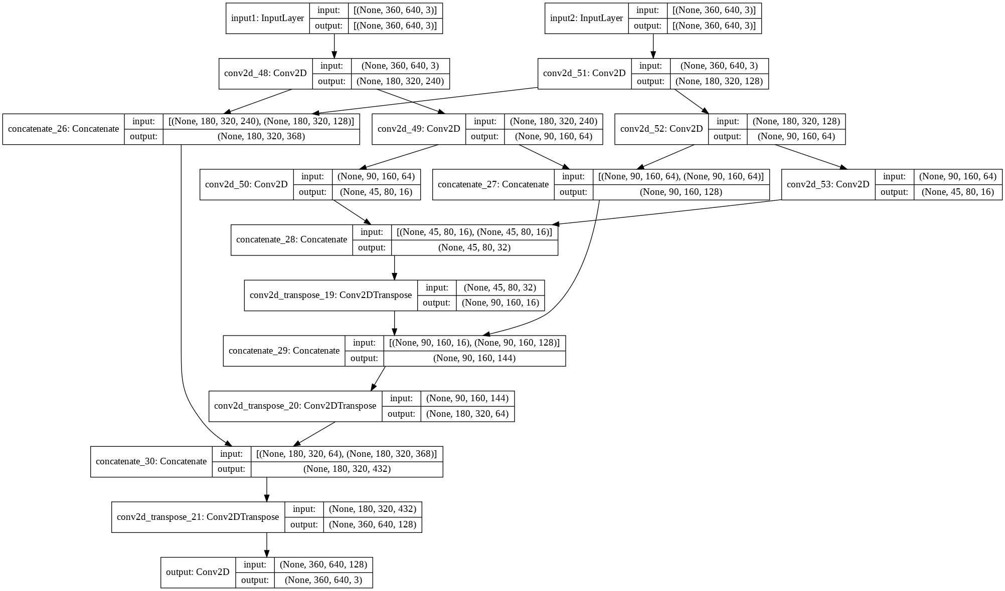
Here we take our previous two input model and have to add a good bit for the skip layers to work. The method I went with was first concatenating the respective layers of the encoders for both the frames. Then I took that concatenated layer and concatenated it with the respecting decoder layer.
As you can see with the easy-to-read diagram below it worked flawlessly.
frame_0_input     = layers.Input(shape=(height, width, channels), name="input1");
f0_0              = layers.Conv2D(240, (3,3), activation='relu', padding='same', strides=2)(frame_0_input)
f0_1              = layers.Conv2D(64, (3,3), activation='relu', padding='same', strides=2)(f0_0)
frame_0_output    = layers.Conv2D(16, (3,3), activation='relu', padding='same', strides=2)(f0_1)

frame_1_input     = keras.Input(shape=(height, width, channels), name="input2");
f1_0              = layers.Conv2D(128, (3,3), activation='relu', padding='same', strides=2)(frame_1_input)
f1_1              = layers.Conv2D(64, (3,3), activation='relu', padding='same', strides=2)(f1_0)
frame_1_output    = layers.Conv2D(16, (3,3), activation='relu', padding='same', strides=2)(f1_1)

combined_0 = layers.concatenate([f0_0,f1_0])
combined_1 = layers.concatenate([f0_1,f1_1])

c0 = layers.concatenate([frame_0_output,frame_1_output])

c1 = layers.Conv2DTranspose(16, kernel_size=3, strides=2, activation='relu', padding='same')(c0)
cx1 = layers.concatenate([c1, combined_1])

c2 = layers.Conv2DTranspose(64, kernel_size=3, strides=2, activation='relu', padding='same')(cx1)
cx2 = layers.concatenate([c2, combined_0])

c3 = layers.Conv2DTranspose(128, kernel_size=3, strides=2, activation='relu', padding='same')(cx2)
frame_0_output = layers.Conv2D(3, kernel_size=(3,3), activation='relu', padding='same', name="output")(c3)

two_input_autoencoder_skip = keras.Model(
    inputs=[frame_0_input, frame_1_input],
    outputs=[frame_0_output],
)

keras.utils.plot_model(two_input_autoencoder_skip, google_drive_path+ "multi_input_autoencoder.png", show_shapes=True)
Setup the Optimizer and Compile
Same as before.
# initiate Adam optimizer
opt = tf.keras.optimizers.Adam(learning_rate=0.00007, beta_1=0.9, beta_2=0.999, epsilon=1e-08)
two_input_autoencoder_skip.compile( optimizer=opt, metrics=[PSNR,SSIM], loss=losses.MeanSquaredError())
Create loop which loads partial data, trains model, and stores results.
Same as before. ( Two Input Model )
block_amount = 10
block_size = 50

two_hist_skip_loss = []
two_hist_skip_psnr = []
two_hist_skip_ssim = []

for block in range(0,block_amount) :
  # Create X and Y Train Arrays
  x_train_0 = []
  x_train_1 = []
  y_train = []

  print("Loading Block: " , block)
  for i in range(0,block_size) :

    # Grab Frame 0,1,2
    print("Grabbing Frame: " , ((block_size * block) + i) )
    img0 = cv2.imread(google_drive_path + "out_frame/frame%d.jpg" % ((block_size * block) + i))
    img1 = cv2.imread(google_drive_path + "out_frame/frame%d.jpg" % ((block_size * block) + (i+1)))
    img2 = cv2.imread(google_drive_path + "out_frame/frame%d.jpg" % ((block_size * block) + (i+2)))

    x_train_0.append((img0/255))
    x_train_1.append((img2/255))
    y_train.append((img1/255))

  print("Loaded Block: " , block)
  x_train_0_np = np.array(x_train_0)
  x_train_1_np = np.array(x_train_1)
  y_train_np = np.array(y_train)

  historyObj = run_model_iteration(two_input_autoencoder_skip,
                                   {"input1": x_train_0_np, "input2" : x_train_1_np},
                                   y_train_np,
                                   512,
                                   4)
  print("Trained Block: " , block)

  two_hist_skip_loss = two_hist_skip_loss + historyObj['loss']
  two_hist_skip_psnr = two_hist_skip_psnr + historyObj['PSNR']
  two_hist_skip_ssim = two_hist_skip_ssim + historyObj['SSIM']

np.save(google_drive_path+"two_hist_skip_loss" , two_hist_skip_loss)
np.save(google_drive_path+"two_hist_skip_psnr" , two_hist_skip_psnr)
np.save(google_drive_path+"two_hist_skip_ssim" , two_hist_skip_ssim)
Graph the Training History
Now we compare the two input skip model to the previous two input model.
two_hist_loss = np.load(google_drive_path+"two_hist_loss.npy")
two_hist_skip_loss = np.load(google_drive_path+"two_hist_skip_loss.npy")

# plot loss
fig, ax1 = plt.subplots()

ax1.plot(two_hist_loss, label='loss', color='tab:blue')
ax2 = ax1.twiny()
ax2.plot(two_hist_skip_loss, label='loss', color='tab:red')

plt.savefig(google_drive_path+ "two_input_skip_model_loss.png")
plt.show()

Blue - Non Skip Model, Red - Skip Model
two_hist_psnr = np.load(google_drive_path+"two_hist_psnr.npy")
two_hist_skip_psnr = np.load(google_drive_path+"two_hist_skip_psnr.npy")

# plot psnr
fig, ax1 = plt.subplots()

ax1.plot(two_hist_psnr, label='psnr', color='tab:blue')
ax2 = ax1.twiny()
ax2.plot(two_hist_skip_psnr, label='psnr', color='tab:red')

plt.savefig(google_drive_path+ "two_input_skip_model_psnr.png")
plt.show()
Here we have the same issue as the two input model before (Having inf PSNR), however we can see that the skip model does eventually get higher.

Blue - Non Skip Model, Red - Skip Model
two_hist_ssim = np.load(google_drive_path+"two_hist_ssim.npy")
two_hist_skip_ssim = np.load(google_drive_path+"two_hist_skip_ssim.npy")

# plot ssim
fig, ax1 = plt.subplots()

ax1.plot(two_hist_ssim, label='ssim', color='tab:blue')
ax2 = ax1.twiny()
ax2.plot(two_hist_skip_ssim, label='ssim', color='tab:red')

plt.savefig(google_drive_path+ "two_input_skip_model_ssim.png")
plt.show()

Blue - Non Skip Model, Red - Skip Model
Here we see that the two input skip model did even better with the higher SSIM value.
Visualize the Results
Same as before.
x_train_0 = []
x_train_1 = []
y_train = []

for i in range(0,30) :
  # Grab Frame 0,1,2
  img0 = cv2.imread(google_drive_path + "out_frame/frame%d.jpg" % + i)
  img1 = cv2.imread(google_drive_path + "out_frame/frame%d.jpg" % + (i+1))
  img2 = cv2.imread(google_drive_path + "out_frame/frame%d.jpg" % + (i+2))

  # We want to train the model to predict differance to the next frame from the differance of the 0 and 2 frames
  x_train_0.append((img0/255))
  x_train_1.append((img2/255))
  y_train.append((img1/255))

x_train_0_np = np.array(x_train_0)
x_train_1_np = np.array(x_train_1)
y_train_np = np.array(y_train)

pred = two_input_autoencoder_skip.predict(  {
                                        "input1" : np.array([x_train_0_np[15]]),
                                        "input2" : np.array([x_train_1_np[15]])
                                        }
                                      )

plt.imshow(pred[0])
plt.show()  # display it

Predicted
plt.imshow(y_train[15])
plt.show()  # display it

Actual
pred = two_input_autoencoder_skip.predict(  {
                                        "input1" : np.array([x_train_0_np[15]]),
                                        "input2" : np.array([x_train_1_np[15]])
                                        }
                                      )

b_pred,g_pred,r_pred = cv2.split((pred[0] - y_train[14]))
fig, axs = plt.subplots(ncols=3,figsize=(100,20))
sns.heatmap(r_pred, ax=axs[0], vmin=-1, vmax=1)
sns.heatmap(g_pred, ax=axs[1], vmin=-1, vmax=1)
sns.heatmap(b_pred, ax=axs[2], vmin=-1, vmax=1)

Predicted Difference
b_act,g_act,r_act = cv2.split(y_train[15] - y_train[14])
fig, axs = plt.subplots(ncols=3,figsize=(100,20))
sns.heatmap(r_act, ax=axs[0], vmin=-1, vmax=1)
sns.heatmap(g_act, ax=axs[1], vmin=-1, vmax=1)
sns.heatmap(b_act, ax=axs[2], vmin=-1, vmax=1)

Actual Difference
r_amp = r_act - r_pred
g_amp = g_act - g_pred
b_amp = b_act - b_pred

fig, axs = plt.subplots(ncols=3,figsize=(100,20))
sns.heatmap(r_amp, ax=axs[0], vmin=-1, vmax=1)
sns.heatmap(g_amp, ax=axs[1], vmin=-1, vmax=1)
sns.heatmap(b_amp, ax=axs[2], vmin=-1, vmax=1)

Difference between Actual and Predicted
Looking mostly at the Difference heatmap and the high SSIM values I believe the two input skip model is the best we got. So its time to make some videos with our new model.
Using CV2 to Export Upscaled / Compressed Video
We need to make a loop which:
Grabs the data frames.
Formats the data for the model.
Generate frames.
Puts frames together in the correct order.
So we want to create a video which:
Is half-speed at 12.5 fps. (100% Original Frames)
Is full-speed at 25 fps (100% Original Frames)
Is full-speed at 25fps but every other frame is replaced with a predicted frame. (50% Original Frames)
A double speed 50 fps video showing upscaling capabilities. (50% Original Frames)
A double speed 50 fps using only 25% original frames (25% Original Frames)
I include recreating the original video because we want a level playing field for comparison. This just creates an optimal control to compare against.
I’m just going to put all of the code down and then have a summary video at the end to have better side-by-side comparisons.
The half-speed video at 12.5 fps.
# Normal 15 fps Video
fourcc = cv2.VideoWriter_fourcc(*'XVID')

img=[]
# Add in every other frame
for i in range(0,250):
    img.append(cv2.imread(google_drive_path + "out_frame/frame%d.jpg" % (i*2)))
    print("adding", i)

height,width,layers=img[1].shape

# Define it with half the fps
video=cv2.VideoWriter(google_drive_path + 'normal_12_5_video.avi',fourcc,12.5,(width,height))

for j in range(0,250):
    video.write(img[j])

cv2.destroyAllWindows()
video.release()
The full-speed video at 25 fps.
# Normal 25 fps Video
fourcc = cv2.VideoWriter_fourcc(*'XVID')

# Read in every frame
img=[]
for i in range(0,500):
    img.append(cv2.imread(google_drive_path + "out_frame/frame%d.jpg" % i))
    print("adding", i)

height,width,layers=img[1].shape

# Define it with full fps
video=cv2.VideoWriter(google_drive_path + 'normal_25_video.avi',fourcc,25,(width,height))

for j in range(0,500):
    video.write(img[j])

cv2.destroyAllWindows()
video.release()
The predicted full-speed video at 25fps .
end_frames = []

fourcc = cv2.VideoWriter_fourcc(*'XVID')

# Read in half of the frames
img=[]
for i in range(0,250):
    base_frame = (i*2)

    # Get Base Frame
    img0     = cv2.imread(google_drive_path + "out_frame/frame%d.jpg" % base_frame)  ;
    img0d    = img0/255;

    # Get Base Frame + 2 for Prediction
    img2     = cv2.imread(google_drive_path + "out_frame/frame%d.jpg" % (base_frame+2));
    img2d    = img2/255;

    # Calculate the predicted diff to the middle frame
    diff = two_input_autoencoder_skip.predict(  {
                                        "input1" : np.array([img0d]),
                                        "input2" : np.array([img2d])
                                        }
                                      )

    #print("Predicted: ",diff[0])
    #plt.imshow(diff[0])

    # Create Center Predicted Frame
    to_add = (diff[0] * 255)
    to_int_clip = np.clip(to_add,0,255)
    to_int_clip_CENTER = np.array(to_int_clip).astype(np.uint8)

    # Add Base Frame
    img.append(img0)
    # Add Predicted Frame
    img.append(to_int_clip_CENTER)
    # So our final ratio of predicted to actual frames will be 1:1

    print("interpreting: ",base_frame+1)

height,width,layers=img[1].shape
video=cv2.VideoWriter(google_drive_path + 'replaced_25_video.avi',fourcc,25,(width,height))

for j in range(0,500):
    video.write(img[j])

cv2.destroyAllWindows()
video.release()
The predicted double-speed video at 50fps.
end_frames = []

fourcc = cv2.VideoWriter_fourcc(*'XVID')

# Read in every frame
img=[]
for i in range(0,500):
    base_frame = i

    # Get Base Frame
    img0     = cv2.imread(google_drive_path + "out_frame/frame%d.jpg" % base_frame);
    img0d    = img0/255;

    # Get Base Frame + 2 for Prediction
    img1     = cv2.imread(google_drive_path + "out_frame/frame%d.jpg" % (base_frame+1));
    img1d    = img1/255;

    # Calculate the predicted diff to the middle frame
    diff = two_input_autoencoder_skip.predict(  {
                                        "input1" : np.array([img0d]),
                                        "input2" : np.array([img1d])
                                        }
                                      )

    # Create Center Predicted Frame
    to_add = (diff[0] * 255)
    to_int_clip = np.clip(to_add,0,255)
    to_int_clip_CENTER = np.array(to_int_clip).astype(np.uint8)

    # Add Base Frame
    img.append(img0)
    # Add Predicted
    img.append(to_int_clip_CENTER)
    # Here we still have the 1:1 ratio, however have double the frames for double the fps.

    print("interpreting: ",base_frame+1)

height,width,layers=img[1].shape
video=cv2.VideoWriter(google_drive_path + 'up_replaced_50_video_fixed.avi',fourcc,50,(width,height))

for j in range(0,1000):
    video.write(img[j])

cv2.destroyAllWindows()
video.release()
The double speed 50 fps using only 25% original frames
end_frames = []

fourcc = cv2.VideoWriter_fourcc(*'XVID')

img=[]
for i in range(0,250):
    base_frame = (i*2)
    # Get Base Frame
    img0     = cv2.imread(google_drive_path + "out_frame/frame%d.jpg" % base_frame)  ;
    img0d    = img0/255;

    # Get Actual Image for Stat Collection
    img_real = cv2.imread(google_drive_path + "out_frame/frame%d.jpg" % (base_frame+1));

    # Get Base Frame + 2 for Prediction
    img2     = cv2.imread(google_drive_path + "out_frame/frame%d.jpg" % (base_frame+2));
    img2d    = img2/255;

    # Calculate the predicted diff to the middle frame
    diff = two_input_autoencoder_skip.predict(  {
                                        "input1" : np.array([img0d]),
                                        "input2" : np.array([img2d])
                                        }
                                      )

    # Create Center Predicted Frame
    to_add = (diff[0] * 255)
    to_int_clip = np.clip(to_add,0,255)
    to_int_clip_CENTER = np.array(to_int_clip).astype(np.uint8)
    to_int_clip_CENTERd = diff[0]

    # Predict Frame Left of Center ( Brand New Frame )
    # Calculate the predicted diff to the middle frame
    diff = two_input_autoencoder_skip.predict(  {
                                        "input1" : np.array([img0d]),
                                        "input2" : np.array([to_int_clip_CENTERd])
                                        }
                                      )
    to_add = (diff[0] * 255)
    to_int_clip = np.clip(to_add,0,255)
    to_int_clip_LEFT = np.array(to_int_clip).astype(np.uint8)

    # Predict Frame Right of Center ( Brand New Frame )
    diff = two_input_autoencoder_skip.predict(  {
                                        "input1" : np.array([to_int_clip_CENTERd]),
                                        "input2" : np.array([img2d])
                                        }
                                      )
    to_add = (diff[0] * 255)
    to_int_clip = np.clip(to_add,0,255)
    to_int_clip_RIGHT = np.array(to_int_clip).astype(np.uint8)

    # Add Base Frame
    img.append(img0)
    # Add Predicted Left
    img.append(to_int_clip_LEFT)
    # Add Predicted Frame
    img.append(to_int_clip_CENTER)
    # Add Predicted Right
    img.append(to_int_clip_RIGHT)

    print("interpreting: ",base_frame+1)

height,width,layers=img[1].shape
video=cv2.VideoWriter(google_drive_path + 'up_replaced_predict_50_video.avi',fourcc,50,(width,height))

for j in range(0,1000):
    video.write(img[j])

cv2.destroyAllWindows()
video.release()
And here are our results. I would recommend only looking at two adjacent ones at a time as its dizzying to look at them all at once.
Conclusions
Overall I was pleased with the results. We were able to make a model which did its job predicting believable frames, and from my initial experiments, I can tell you getting that working isn't as easy as it seems. I wonder if the two-input skip model is better because of its increased complexity and not because it truly is a better representative architecture. To approach that question, we would have to start training and testing these models over multiple videos. (and no one has time for that)
Looking at the video I am most pleased with the upscaled version with 50% original frames. The camera pan over the building looked a lot smoother. I was also surprised how well the 25% original frame version worked out. It was still jittery but it’s neat that it’s mostly predicted information. Then the 25 fps version in my eyes looked a tad bit better than just deleting every other frame (12.5 fps version) but again was jittery.
One disappointment is that I tried to get this working with a Quantized Neural Net using the Larq package; however, the model kept converging to very small values. When I could get a frame out, it was too low quality to compress or upscale a video effectively. But that does leave something to try out in the future.
In the end, I'm at least now able to grasp some of the ideas that these papers are touching on, and that was the entire point of this exercise. So that's a win in my book.
I hope you enjoyed reading, and if you have any questions, feel free to reach out.