Using Reinforced Learning to Create Efficient Random Tests
A final project for Verification class. Worked with Ayushi Trivedi, and the class was taught by Monica Farkash.
Introduction
A large part of my job as a design engineer is to help enable coverage closure for the designs I own. For readers unfamiliar with software or hardware coverage, it's just the measure of how many lines of code were run and conditions taken in all of the tests of a particular design. When a team is satisfied that all the tests cover enough of the design, it can be used as evidence that you made something work that won't break once it goes into the real world.
In my experience, achieving coverage closure involves two main stages: before and after ~80% of coverage. The majority of the engineer's time is spent on the complex, challenging work to get that last (20%) percentage of coverage, whereas the work to get the first chunk (80%) of coverage is mostly a matter of running more, longer tests or tests with a lot of randomness. However, while efficient in terms of engineering hours, this simple solution of running more tests to get this large chunk has limitations. It consumes significant computational time and power, especially with designs with high configurability, where this process has to be repeated multiple times.
There have been steps to solve the volume problems that come with random testing, such as constrained stimulus, where the tests use stimulus with a particular distribution to cover more significant cases. This method helps but fails because sometimes sequences of transactions are needed to get closure more often than just specific lines of stimulus. Saving a particular test seed with high coverage and running those helps; however, once a design changes, these seeds become less effective. Additionally, when conditions are challenging, we often have to start making directed tests. Still, many of these difficult-to-hit conditions exist, so creating a directed test each time isn't viable or sustainable. What you are left with at the end of this is running thousands of tests, each with tens of thousands of cycles, just to be able to cover some select difficult conditions, which at the end of the day can be an inefficient use of compute time or resources.
The Approach
With trying to use reinforced learning for everything, I felt there should be some way to make an intelligent agent that can create random stimuli more thoughtfully, primarily because data generated from all of this verification effort can be used to help teach an agent to help us with this. The first branch one may look at is whether a reinforced learning agent can look at the design itself and generate an optimal test. An agent can learn how to toggle the inputs to cover the design by looking at the inner gates, wires, and connections (or RTL code). This methodology would allow an agent to understand any design as the agent can look at any arbitrary set of gates and wires. However, this has a vast state space problem; the different design possibilities will quickly grow, meaning the state space an agent looks at is large. Then, suppose there isn't any context to the input wires to the design. In that case, the possible actions the agent could take will also grow exponentially as input buses widen.
Thinking further, we must find a way to reduce the complexity. Having an agent that can take in any possible RTL design and output a full-fledged random test doesn't pass the high-level sniff test in terms of doability. So, there are two things to simplify: the state space the agent looks at and what the agent generates.
As for what the agent generates, let's reduce it to just one line of stimulus or one action. So, instead of outputting a test that runs hundreds of actions, give one action to maximize coverage for a particular state. This means that the agent will have to run multiple times to generate a more significant test; however, that will take significantly less time than trying to train an agent who makes the more extensive test in one shot. So, running an agent 100 times to make a 100 command test will be a faster way to find a solution than making an agent that can run once to create a 100 command test.
One way to simplify the state input is to stop thinking that this agent can work for every design but would need to be trained for each individual design. This is less costly than one might think, as each design is already running thousands of tests anyway for coverage closure (sometimes every day), so using these cycles for coverage and training the agent simultaneously is a realistic possibility.
If that is the case, then deep down, we have to understand what we truly want the agent to do. We want an agent to give us the most efficient action to get as much coverage as possible. To do this, the agent needs to look at what's already covered to generate an action to target what isn't covered. In addition, having a history of the commands could help the agent learn how different sequences could be used to address holes in the coverage. (Note: This project mostly runs agents that don't have command history, but an experiment towards the end of this write-up does have it.)

Figure 1: The High Level Idea Behind a Smart Agent. Red == Not Covered, Green == Covered
So, we are left with an agent that looks at coverage points for a specific design searching for holes and possibly previous commands to understand what has been done in the past. In that case, it should generate a new action to close the most additional coverage. While the state space is still significant, it can be manually or algorithmically experimented with to be reduced, whether selecting interesting coverpoints or focusing only on specific inputs. If the agent was generic versus trained for a particular design, it would be challenging to know what parts of the generic RTL design to trim to reduce the state space. However, it is possible for a human (or a computer) to find essential coverage points in a specific design and only use those for the state calculation.
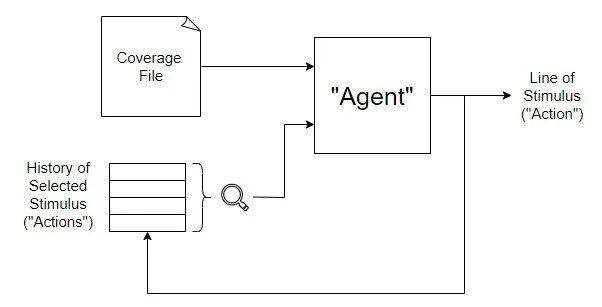
Figure 2: Top Level Diagram of an Agent
Ultimately, we want to create an intelligent agent that can look at the current state of coverage and the history of actions to give us the optimal following action to close the most coverage. This agent can then be run multiple times, looking at the coverage after each command to generate more extended tests. Randomness can still come into play by having the agent only make an intelligent decision sometimes. So, one can still create a suite of random tests and not just have the agent create the same test based on the same initial condition.
Another Problem
Another problem arises just from looking at previous reinforced learning projects: It will take millions, or at least hundreds of thousands of games, to make an agent that can learn properly. The issue is that most of the tools to run coverage must compile the RTL design, simulate the test, and then collect coverage. This cycle takes at least a minute or two for most tools, even for minimal designs. Using classical (heavy-duty) tools will take years to run experiments of this length. We need to find a way to run coverage experiments many orders of magnitude faster. (or actually, build it in the tool itself, which isn't possible as these are closed-source tools, and we would have needed more time to explore a route that complex.)
To do this, Verilator comes to the rescue. This tool allows us to compile a C++ testbench of the RTL into a single executable. It also has a feature enabling us to measure coverage, which works well enough for some initial testing purposes. You could also use many other great tools like cocotb to explore like this. Still, the key is that this sort of training needs something that can run with a lighter weight than many of our primary tools.
This executable that Verilator builds will take in stimulus from an external text file and drive the block's input pins using that stimulus. This allows us to have quicker training cycles. More details about how the testbench is set up will appear later in this write-up.
High-Level Learning Cycle
The cycle of learning for the agent will look like this:
Look at the coverage of a design and previous actions. (Initially empty data.)
Choose an action with some epsilon (randomness).
Convert the action to 1s and 0s to drive the input signals
Append that to a stimulus file.
Run the Verilator executable file.
Read the coverage file to see how much coverage was achieved.
Finally, use this coverage as a reward for an action state pair.
Go to 1 with the updated coverage and action history.
At the end of the day, reading the coverage file and running Verilator took about equal time. With this reduced run time, we could run a full round in less than half a second. The reduction in time allows for long experimental runs that can finish overnight and, more extensive, final runs that take a day or two, which is more realistic.
Now that we have a high-level idea of the training cycle and what tools we can use to extract coverage, we need to look for some designs to experiment on and set up the testbench.
Finding Designs, Defining Actions, and Setting up the Testbench
For some initial designs, we need ones with a relatively high complexity where coverage closure isn't some trivial combination of inputs. Secondly, having a smaller input action space allows the agent to learn only a few actions. This combination is an ideal way to see if this idea has any legs.
Suitable candidates that were found were a BTB (Branch Table Buffer), an Instruction Cache, and a Data Cache. These designs have a relatively large space to cover, but the inputs to the block are a smaller action space. We abstract to this action space because the state space for selecting specific inputs for even 32 binary input bins would be significant. Instead, if we use actions such as "A write occurs to a recently used address," we can define a space order of magnitude smaller for the reinforced agent to learn.
The action space of each of these blocks is below:
BTB (385 Actions. An action will have a selection of each item below):
Branch Request (0 or 1)
Invalidate (0 or 1)
PC Accept (0 or 1)
Taken (0 or 1)
Call, Return, or Jump (0, 1, or 2)
Source/FI (0 or 1) : Random PC or Previous PC
Program Counter (0, 1, 2, or 3) : Random Address, Previous Address Plus 4, Historic Address Minus 4, HistoricAddress Minus 8
Instruction/Data Cache (8/32 Actions):
Enable/Disable Cache (0 or 1)
Read from an Address (0, 1, 2, or 3): Random Address, Previous Address Plus 4, Historic Address Plus 64, Historic Address with Different Tag
(Data Cache) Write to an Address (0, 1, 2, or 3): Random Address, Previous Address Plus 4, Historic Address Plus 64, Historic Address with Different Tag
So, instead of having the agent try to learn arbitrary bit inputs, which is needed if it is generic for any design, we can take hints from the design itself to construct a reduced action space with relevant stimulus to what is being verified. These actions selected will map to specific 1s and 0s that can drive the design inside the testbench. Now, how do we drive the design?
The testbench is a barebones C++ Verilator testbench, at the end of the day. It looks at a stimulus file line by line and drives the inputs according to the stimulus file. The agent building this stimulus file will provide all the smarts for driving the block's input. This file back-and-forth is just used as a communication instrument between the agent and the Verilator testbench.
Future work could be done to see if the agent can be made in C++ and incorporated into the Verilator bench itself so there won't be a need to read/write all of these files for communication. (Which takes up more than half the training time). As described later, the training and executable coordination will be done in Python.
Good place to start with Verilator and Coverage: https://github.com/verilator/example-systemverilog
An example testbench file is below (started from example template in repository) :

Figure 3: The Top Level C++ Verilator Bench (From Data Cache)
The RTL bench mainly consisted of the just the DUT. However, it should be noted that the data cache had more logic added to it with an open-source AXI Memory Emulator, which was needed since it required interaction with a more complicated AXI interface to operate correctly. The instruction cache interface was more straightforward, and two signals had to be tied to 0 because of the simple handshake of the internal bus used. The BTB also didn't need any additional logic inside the testbench to get it running.
Now, we have the setup to generate a couple of Verilator executables that can run a stimulus file on an RTL design and output coverage information. It's on to defining the agent and the environment at a high level to start coding.
Defining the State, Reward Function, and when a Test is Done
State the Agent Will Observe
At first, we tried to use the percentage coverage quantized to some number of bits as the state. For example, a 2-bit quantized state with 23% Line Coverage, 78% Conditional, and 55% Toggle will reduce to [00,11,10], which is six bits of state. Our initial runs were done with about 16 total bits (some coverage types were given more quantization than others), making a state space of 64k possible states. This state space provided some promise, but learning was very noisy and didn't progress significantly, so other options were explored quickly.
The next stage we tried was the actual coverage vector, meaning that each coverage point would take up a "bit" of space (1 [Covered] or 0 [Uncovered]). These designs had about 500 to 3.5k coverage points, so the state space is quite large, meaning some state space reduction would be an area to explore further. However, this project just took this vector at face value.
After this, the past commands are appended to the end of this coverage vector, so an array will be appended to the bit vector, which contains the previous action numbers. For example, if there are 300 possible actions, an action history will look like [23, 283, 21, ...]. So the state will look like : [0,1,0,1,1,...,0,1,23, 283, 21,33,33]
The agent will then consist of multiple DNNs that look at this state vector and produce a value that is an expected reward. Each possible action will have its own DNN, meaning that a DNN's responsibility is to look at the current state and give an expected reward for a specific action. The last step would be to choose the action associated with the DNN with the most significant expected reward.
When is the game done?
For these experiments, the number of cycles a test ran was just a predefined number, meaning a test with 100 cycles of stimulus or a test with 1000 cycles of stimulus. Each step of the game involved the agent selecting a stimulus cycle for a given state observed. At first, we tried to have 100% coverage be the point an individual game was done; however, this wasn't guaranteed to ever happen for both coding and tooling reasons. So, the focus was to bind the test to some known number and see how the agent would do.
Rewards
The rewards had a significant problem from the beginning, and it deals with that idea I talked about toward the top of this write-up. The initial large chunk of coverage is easy to get with randomness, while the harder last bits need more effort. This is an issue because the training is very noisy if we use plain coverage as a reward. The agent can do whatever it wants to get these large initial rewards. So the reward function was made into an exponential curve, so the hardest last bits of coverage counted as more of a reward. Additional experimentation was done to give more or less weight to types of coverage, which also helped depending on the specific design that was running. Overall, what was found is that it is essential to learning the reward consists mainly of valuable, more complex coverage points in terms of the magnitude of contribution.
Now, the timing of these rewards is also essential. You could give a reward for the difference in coverage gained from adding that line of stimulus to the file (essentially each round of a game); however, this didn't work very well. Instead, all the rewards come at the end of a game. Only when the game is done will the Agent get a reward. This means that only state action pairs common to the end of a test will initially see a reward.
But as more games are played, this reward will backpropagate to state action pairs that are more common at the beginning of the test. Again, this is typically very noisy because of the extensive coverage gains of running a couple of random stimulus lines.
The Agent Architecture
The agent is in charge of analyzing an environmental state and converting it into an action, which is typically done through learned Q-Functions. These functions try to find the expected future rewards for all actions. For this project, a separate Q-Estimator was created for each action. So, each action's estimator would provide an expected reward based on the current state. The agent will then act with the highest expected reward.

Figure 4: Inside an Agent
This project explored using the SGDRegressor and the MLPRegressor to convert the state to an expected reward. Both had trouble converging initially, so much hyperparameter tuning and analysis of the gradient decent values was needed. SGD needed a good amount of regularization with alphas from 0.6 to 5 with relatively small learning rates. Then, the MLP regressor was sensitive to the size of the hidden layers. If it was too large, the weights had trouble converging. If it was smaller, it limited the learning it could eventually achieve. No real hard and fast rules came out of this project. Still, it did show it is possible that the agent could not learn at all unless the correct hyperparameters were found, so if it doesn't work initially, some deep dives need to happen to understand why the functions aren't covering.
The Python Code
All of the orchestration and reinforced learning cycles were done in Python at the top level. The following sections go through the code, explaining what is happening.
The Training Loop and Epsilon Calculations
The main training loop was relatively simple. The agent will play a game on the environment for several runs. In this case, one game would be a full test. So, if we train it for one hundred thousand runs, it is taught by creating a hundred thousand tests and seeing how well it did closing coverage with those tests.
In each game loop, epsilon is first calculated, starting high and gradually reducing. Epsilon is the amount of randomness the agent takes. In the beginning, the agent will explore more and later optimize the best ways it found to close coverage by injecting less randomness.
This epsilon function was a significant factor in how well the agent learned. It took a good bit of tuning and experimentation to get a good epsilon, which would provide the agent with enough exploration before it started the optimization phase. If it stopped exploring too quickly, it would fail to learn and generally degrade once it reached a certain point of epsilon. If epsilon didn't lower fast enough many times, the agent would get too optimized for specific state spaces it might not see and have trouble relearning once epsilon goes down. Both of these led to learning degradation earlier on after higher epsilon values.
The inner game loop iterates each turn of this game, where the agent chooses individual commands to provide stimulus to build up the test. This loop is when the agent looks at the environment, chooses a stimulus, updates the environment, and the environment provides back a coverage score for the agent to learn. This is done until the test is made, and then the environment is reset so the agent can go through another test.
We also had a bunch of logging and checkpointing throughout this code.

Figure 5: The Main Training Loop (Hardware Agnostic)
The Environment
The environment has several methods, mainly init, step, and reset. Init initializes the internal state, and for this project, it will be an empty coverage vector with the addition of an empty command history. Step is what takes in the action, will update the stimulus file, run the verilator executable, read the coverage from the run, and return the reward based on the results. In addition, will provide the done signal for when a test is deemed to be done. The reset method is similar to the init method in that it reinitializes the environment to run for another test.

Figure 6: The Environment (Data Cache)
The Function Approximatior
This class is in charge of initializing the models for each of the actions and then providing a predict and update method. The predict method can take in a state and output expected future rewards (q-values) for each of the actions. The update function can look up an action model and train it with the reward that was returned for a specific state.
This class is really what the "Agent" is. It was saved and checkpointed during the learning process, as it contains the models with all of the learning smarts. The external logic is just structural to help this Approximator learn.

Figure 7: The Agent (Hardware Agnostic)
Policy
This code just takes in the q-values for the actions and an epsilon to decide what action to take.

Figure 8: The Policy (Hardware Agnostic)
Run Verilator and Read Coverage Method
This method runs the Verilator bench, which takes in the stimulus file to drive the dut's input pins.

Figure 9: Running Verilator (Hardware Agnostic)
This method goes through the coverage log from the Verilator run and can return a coverage vector.

Figure 10: Reading Coverage (Hardware Agnostic)
Declare and Run
How to create objects and start training:

Figure 11: Start the Learning (Data Cache)
Evaluation Methodology
For each hardware module, we looked at three main things. First is the ability of the agent to learn based on the decrease in epsilon. This can be shown in a plot of the score the agent can achieve versus the epsilon at the moment. (Or plot coverage closure as epsilon decreases)
Secondly is the per-test coverage amount. Ideally, each test can be made more efficient, covering more of the code than random stimulus. This is done by generating hundreds of tests at different epsilons. Then, the coverage is measured for each test and plotted to show how the average test coverage changes based on the epsilon of the agent. (0 would be no randomness, 1 would be only random choices, and 0.5 would be making a random decision half of the time)
Finally, there is the inter-test coverage. Ideally, better coverage can be achieved earlier in each test. To measure this, hundreds of tests are again generated; however, we also collect the amount of coverage that is closed each cycle of the test. By comparing across epsilon, we can see if more coverage is achieved on average earlier in each individual test.
These measurements show that, on average, you get more coverage per test and that, within each test itself, more lines will be covered sooner.
General Observations
One general observation of all the runs was a gradual increase in the score as the epsilon was lowered. However, there was typically a point where the agent would quickly degrade if epsilon got too low. This led to saving optimal models along the learning process, but also during evaluation different epsilons were looked at to see how effective randomness could be used with the smarts of an agent in combination. Running the agent with a mid-range (0.5) epsilon can give some improvements over pure random and also better results than having an agent with no randomness included in some cases.
Another observation is that even though the score is noisy and sometimes looks like the agent hasn't done an excellent job learning, the results from the actual evaluation show significant improvements over pure random. This points to the fact that the current score calculated may not be the best learning indicator and could use improvement. Targeting more critical lines of coverage for the score would be a better indicator.
Branch Target Buffer
The BTB ended up being a well-behaving first case to examine. It could learn at a constant rate until epsilon reached about 0.4, meaning the agent made a smart decision most of the time. One note to make also is that the BTB agent did NOT use the stimulus history when generating new lines of stimulus.
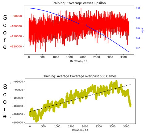
Figure 12: Training Results of BTB
The per-test coverage results aren't as good. The only positive is that the higher epsilon runs had a lower floor than the lower epsilon ones. On average, however, it is very noisy. Luckily, more promising results were seen in the other hardware runs where more parameter tuning had already been done.

Figure 13: Per Test Results of BTB
Some better results can be seen for the inner test coverage plot. Averaging over 100s of tests, the lower epsilon agent shows a decisive advantage in getting more coverage earlier. It is just 10 coverage points (out of ~360) more about cycle 5 of the test. Still, those last coverage points are the most difficult to achieve so even though its a small amount, this can be useful.

Figure 14: Inner Test Coverage for BTB
These results did show some learning for the first run, which was promising. However, the action space is huge, so ideally, reducing that with the instruction cache runs will show more promise.
Instruction Cache
The Instruction Cache was exciting in that it showed no learning (even decreasing) as the epsilon was lowered when we did short runs. But one night, I just let it finish, and there was a very large jump where tests started to, on average, get 5% more total coverage about 12 hours into training. So, this behaved significantly differently from the BTB, which had a more consistent learning trajectory. This sort of behavior indicates that a better reward function may be needed (target important lines better). Once it found a way to make the reward get a reliable jump (or the reward became a reliable measure), it could start learning. Again, the Instruction Cache didn't have the command history to look at when making decisions.

Figure 15: Training Results of ICache
Overall, the ICache had significantly better empirical results. The per-test coverage points with epsilon as low as 0.02 show that more coverage was reached in practically every test over more random agents.

Figure 16: Per Test Results of ICache
Instead of focusing on the inner test results for this bench, I focused on coverage points achieved over time as more tests were run. I made a graph showing accumulated coverage points over multiple tests to do this. These graphs show that after 1000 tests, the agent got about 13% more coverage points overall than just random testing. This provides some evidence that the agent can generate stimulus that can get coverage that random will not be able to achieve for more tests. Also shows proof that the agent is learning a non trivial policy that is better than random selection.

Figure 17: Coverage over Time for ICache
Data Cache
For the Data cache, we did two runs—one with the command history and one without.
Without Command History
It showed similar training results to the BTB, with the constant increase and eventual degradation. One interesting point with the DCache is that the best agents typically have epsilons of 0.6 to 0.8 which is a good amount of randomness. However, even with the large amount of randomness, they could achieve significantly more coverage on average. Averaging over 100 tests, they can reach close to 50 more coverage points (out of 3100)

Figure 18: Training Results for First DCache Experiment

Figure 19: The Converging Average Coverpoints per Test
Looking at the cumulative test coverage, these agents could reach the max coverage point in about 70% fewer tests. In addition, they could get more coverage sooner in the inner test.

Figure 20: Coverage over Time for DCache

Figure 21: Inner Test Coverage for DCache.
With Command History
The training for this was not as well behaved. Still, it did show the same behavior as ICache, where a considerable headway was made in training and then lost. Saving this well-performing model and using an epsilon of 0.65 didn't allow it to behave as well without command history, but it still performed better than an entirely random agent.

Figure 22: Training Results for Second DCache Experiment

Figure 23: The Converging Average Coverpoints per Test
The cumulative coverage showed results similar to those above.

Figure 24: Coverage over Time for DCache
If command history is included, then more training or better methods are needed as commands expand the state space from a bit vector to additional terms, which can be actual integers.
Conclusions
Overall, the results look very promising. We could have done better by staying constant in the evaluation techniques or with the hyperparameters of the runs. But there is enough evidence to set up a more professional thought-out setup and do some week-long training runs to see what happens. Also, more evaluation in terms of compute time saved could have been a good stat to keep track of.
I plan to revise this in the future and add more in terms of optimizing cover points by doing some unsupervised learning so a significantly large state space of coverage points can be reduced to only the important ones. For example, it would be very useful to find the 100 coverage points that, in the end, made the difference in the DCache evaluation versus the initial 3000 that can just be hit with random actions.
Thanks for reading, and if you have any questions, feel free to reach out.
Setup
This was run on Google Collab instances, and also used Amazon EC2 instances. With using MLP it helps having GPUs, otherwise its mostly sequentially bound and you need better CPUs.
Some Sources
Initial RL Code that helped a Ton:
BTB: https://github.com/ultraembedded/biriscv
ICache and DCache were from A57 Core RTL Provided in Class (Not sure about redistribution)